Functions and limits

Calculus is the mathematics of change. Engineers use it to describe how fast a tank fills, how a beam bends under load, how a capacitor charges and how heat flows through a wall. Every one of those ideas rests on a single concept: the limit. Before you can find a rate of change at an instant, or an area under a curve, you need a precise way to say what a function is approaching.

This lesson builds that foundation. You will review functions, learn what a limit means, evaluate limits by several methods, handle limits that involve infinity, and see how limits define continuity. Take your time with it. Everything in the rest of the course is built from these ideas.

Why engineers need limits

Suppose a sensor records the position of a conveyor belt every second. From the data you can easily find the average speed over any interval: distance traveled divided by time taken. But what is the speed at exactly \(t = 3\) seconds? A single instant has zero duration, so the formula "distance divided by time" gives \(0/0\), which means nothing on its own.

The way out is to look at average speeds over shorter and shorter intervals around \(t = 3\): one second, a tenth of a second, a thousandth of a second. If those averages settle toward a single value, that value is the instantaneous speed. "Settling toward a value as the interval shrinks" is exactly what a limit describes.

The same idea appears all over engineering. Stress at a point is the limit of force divided by area as the area shrinks. The current in a wire is the limit of charge passed divided by time. Even the claim that a mathematical model behaves sensibly (that a small change in input produces a small change in output) is a statement about limits, called continuity.

Functions: the raw material

A function is a rule that assigns exactly one output to each allowed input. We write \(y = f(x)\): the input is \(x\), the output is \(f(x)\). The set of allowed inputs is the domain; the set of outputs the function actually produces is the range.

In engineering, functions are models. The deflection of a cantilever beam depends on the load; the pressure in a pipe depends on the flow rate; the temperature of a cooling part depends on time. Writing the relationship as a function lets you analyze it.

A function can be given by a formula, a table of measurements, a graph, or a description in words. Each form has strengths. A formula is easy to manipulate; a table is what you usually get from a test; a graph shows the overall behavior at a glance.

Finding the domain

When a function is given by a formula and nothing else is said, its domain is every real number for which the formula makes sense. Two rules catch most cases: you cannot divide by zero, and you cannot take an even root (such as a square root) of a negative number. Logarithms add a third rule: \(\ln x\) needs \(x > 0\).

Physical models add their own restrictions. A box side length must be positive; a time after a valve opens cannot be negative. Always ask what inputs make sense in the real situation, not only in the formula.

Piecewise functions

Many engineering quantities follow different rules in different ranges. A spring might stretch freely until it hits a stop; an electricity tariff charges one rate up to a threshold and another rate above it; a valve is closed, then ramps open, then stays fully open. These are piecewise functions: one function defined by several formulas, each on its own interval.

Here a spring force \(F\) (newtons) rises at 200 N/m until the extension \(x\) reaches 0.05 m, when the spring hits a much stiffer stop. At \(x = 0.05\) both formulas give 10 N, so the two pieces join up. Whether pieces join or jump is exactly the kind of question limits answer.

Composition

Functions can be chained: the output of one becomes the input of the next. If \(g(x) = x^2 + 1\) and \(f(u) = \sqrt{u}\), then the composition is \(f(g(x)) = \sqrt{x^2 + 1}\). Real systems are full of compositions: temperature depends on time, resistance depends on temperature, so resistance depends on time through a composition. You will need composition again when you meet the chain rule in Lesson 3.

The idea of a limit

Consider the function

At \(x = 2\) the formula gives \(0/0\), so \(f(2)\) is undefined. But we can still ask what happens to \(f(x)\) as \(x\) gets close to 2. Evaluating it at nearby inputs:

• \(f(1.9) = 3.9\), \(f(1.99) = 3.99\), \(f(1.999) = 3.999\)
• \(f(2.1) = 4.1\), \(f(2.01) = 4.01\), \(f(2.001) = 4.001\)

From both sides, the outputs close in on 4. We say the limit of \(f(x)\) as \(x\) approaches 2 is 4, and write:

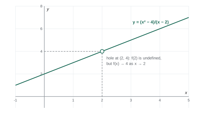
This is the central idea: a limit is about the values a function approaches near a point, not its value at the point. The function might be undefined there, or defined with a different value, and the limit does not care.

In words, \(\lim_{x \to a} f(x) = L\) means we can make \(f(x)\) as close to \(L\) as we like by taking \(x\) close enough to \(a\) (but not equal to \(a\)). Mathematicians make "as close as we like" precise with the ε–δ definition. For engineering calculus, the intuitive version is enough, provided you use it carefully.

One-sided limits

Sometimes a function approaches different values from the left and from the right. We write \(\lim_{x \to a^-} f(x)\) for the limit from the left (inputs less than \(a\)) and \(\lim_{x \to a^+} f(x)\) for the limit from the right.

The two-sided limit exists only when both one-sided limits exist and are equal. If they differ, the limit does not exist, even though each side settles nicely on its own.

Limit laws and direct substitution

Working from tables every time would be slow. Fortunately, limits obey simple algebraic laws. If \(\lim_{x \to a} f(x) = L\) and \(\lim_{x \to a} g(x) = M\), then:

• Sum and difference: \(\lim (f \pm g) = L \pm M\)
• Constant multiple: \(\lim c f = cL\)
• Product: \(\lim (f g) = LM\)
• Quotient: \(\lim (f / g) = L / M\), provided \(M \ne 0\)
• Power and root: \(\lim f^n = L^n\), and \(\lim \sqrt[n]{f} = \sqrt[n]{L}\) (with \(L > 0\) for even \(n\))

Combined with the two basic facts \(\lim_{x \to a} c = c\) and \(\lim_{x \to a} x = a\), these laws give a powerful shortcut. For any polynomial, and for any rational function whose denominator is not zero at \(a\), the limit is found by substituting \(x = a\) directly.

Direct substitution also works for roots, exponentials, logarithms and trigonometric functions at any point inside their domains, because these functions are continuous there (more on continuity below).

Indeterminate forms: when substitution gives 0/0

If direct substitution gives a non-zero number divided by zero, the limit is infinite or does not exist; we will look at that case shortly. If it gives \(0/0\), the result is called an indeterminate form. It does not mean the limit is zero, undefined, or one. It means the expression needs to be rewritten before you can see the answer.

Three algebraic techniques handle most \(0/0\) limits.

Technique 1: factor and cancel

If a polynomial is zero at \(x = a\), then \((x - a)\) is a factor. Factor top and bottom, cancel the common factor (allowed because \(x \ne a\) inside a limit), then substitute.

Technique 2: rationalize

When a square root causes the \(0/0\), multiply top and bottom by the conjugate. This uses \((\sqrt{A} - B)(\sqrt{A} + B) = A - B^2\) to clear the root.

Technique 3: combine fractions

Compound fractions often hide a common factor. Put everything over a common denominator and simplify.

Infinite limits and vertical asymptotes

Consider \(f(x) = \dfrac{1}{x - 2}\) near \(x = 2\). Substituting gives \(1/0\): a non-zero number divided by something approaching zero. The output grows without bound.

• As \(x \to 2^+\), the denominator is a small positive number, so \(f(x) \to +\infty\).
• As \(x \to 2^-\), the denominator is a small negative number, so \(f(x) \to -\infty\).

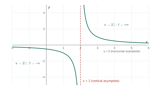
Writing \(\lim_{x \to 2^+} f(x) = \infty\) is a precise description of how the function behaves; it does not mean the limit exists as a number. When a function becomes unbounded as \(x\) approaches \(a\) from either side, the line \(x = a\) is a vertical asymptote.

To find the sign of an infinite limit, check the sign of the numerator and of the denominator just to the left and right of the point. For \(\dfrac{x + 1}{(x - 3)^2}\) near \(x = 3\), the numerator is about 4 and the squared denominator is positive on both sides, so the function goes to \(+\infty\) from both sides.

Vertical asymptotes in a model usually signal a physical limit or a breakdown of the model. The resonance curve of an undamped oscillator has one at the natural frequency, which is why real structures need damping.

Limits at infinity and horizontal asymptotes

Engineers often ask about long-term behavior: what temperature does a part settle to, what speed does a falling object approach, what voltage does a capacitor reach? These are limits as \(x \to \infty\) (or as time \(t \to \infty\)).

The key fact is that \(1/x^n \to 0\) as \(x \to \infty\) for any positive \(n\). For a ratio of polynomials, divide top and bottom by the highest power of \(x\) in the denominator.

This gives three quick rules for rational functions as \(x \to \pm\infty\):

• Degree of top less than degree of bottom: the limit is 0.
• Degrees equal: the limit is the ratio of the leading coefficients.
• Degree of top greater: the function grows without bound (no horizontal asymptote).

Exponential decay to a steady state

Many engineering transients have the form \(A + B e^{-t/\tau}\), where \(\tau\) is a time constant. Because \(e^{-t/\tau} \to 0\) as \(t \to \infty\), these approach the steady value \(A\).

The squeeze theorem and the key trigonometric limit

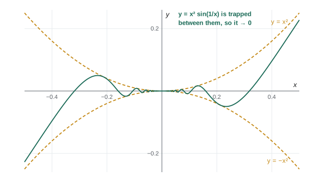
Some limits cannot be simplified algebraically. The squeeze theorem handles many of them: if \(g(x) \le f(x) \le h(x)\) near \(a\), and both \(g\) and \(h\) approach the same limit \(L\), then \(f\) is trapped and must also approach \(L\).

The squeeze theorem also proves one of the most important limits in calculus. With \(x\) in radians:

A geometric argument on the unit circle shows that \(\cos x \le \dfrac{\sin x}{x} \le 1\) for small \(x \ne 0\). Since \(\cos x \to 1\), the ratio is squeezed to 1. In plain terms: for small angles in radians, \(\sin x \approx x\). This is the small-angle approximation used for pendulums, structural rotations and optics. It only works in radians; in degrees the ratio approaches \(\pi/180\), not 1.

Continuity

Informally, a function is continuous if you can draw its graph without lifting your pencil. Formally, \(f\) is continuous at \(x = a\) when three conditions all hold:

• \(f(a)\) is defined;
• \(\lim_{x \to a} f(x)\) exists;
• the two are equal: \(\lim_{x \to a} f(x) = f(a)\).

If any condition fails, \(f\) has a discontinuity at \(a\). There are three main types:

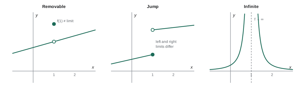
• Removable: the limit exists but \(f(a)\) is missing or different. Redefining one point fixes it, as with the hole in our first example.
• Jump: the one-sided limits exist but differ. A switch closing, a valve slamming shut, or a load suddenly applied produces a jump.
• Infinite: the function is unbounded near \(a\), as at a vertical asymptote.

Polynomials, exponentials, sine and cosine are continuous everywhere. Rational functions, roots, logarithms and tangent are continuous everywhere in their domains. Sums, products, quotients (where the denominator is not zero) and compositions of continuous functions are continuous. This is why direct substitution works so often.

The Intermediate Value Theorem

Continuity has a powerful consequence. If \(f\) is continuous on \([a, b]\) and \(N\) is any value between \(f(a)\) and \(f(b)\), then \(f(c) = N\) for at least one \(c\) between \(a\) and \(b\). A continuous function cannot get from one value to another without passing through every value in between.

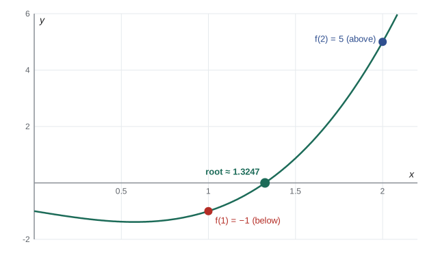
The most common use is finding roots. If a continuous function is negative at one point and positive at another, it must cross zero somewhere between them.

Repeatedly halving the interval like this is the bisection method. It is slow but completely reliable, and engineering software still uses it as a safe fallback. In Lesson 4 you will meet Newton's method, which finds the same root far faster.