Integrals in engineering: beams, fluids and heat

Engineering analysis repeatedly follows the same pattern: a physical law describes what happens in a tiny element of a structure, a fluid or a solid, and integration adds up the elements to give the behavior of the whole. Lesson 3 used this pattern for volumes and work, and Lesson 4 for centroids and moments. This lesson applies it to three areas that every engineering student meets in the second year: the bending of beams, the flow of fluids in pipes and the atmosphere, and the conduction of heat through walls and insulation. In each case, setting up the integral from a small element is the essential skill, and the integration techniques of this course do the rest. The results are classic formulas found in every engineering handbook; deriving them shows where they come from and when they apply.

Loads, shear and bending moment

A beam carries loads across a span. At any section, the material to one side exerts on the other a shear force \(V\) (perpendicular to the beam) and a bending moment \(M\). Considering the equilibrium of a short slice of length \(dx\) carrying a distributed load \(w(x)\) (force per unit length, positive downward) gives two simple relations:

So the shear force is an integral of the load, and the bending moment an integral of the shear force. The constants of integration come from the support conditions: at a simple support or free end, the bending moment is zero; at a free end, the shear force is also zero. The bending moment is largest where the shear force is zero, a direct application of Calculus I.

Deflection of beams

Bending curves a beam. For small deflections \(y(x)\), the curvature is approximately \(y''\), and the Euler-Bernoulli beam theory relates it to the bending moment:

where \(E\) is the modulus of elasticity of the material and \(I\) the second moment of area of the cross-section (Lesson 4). Integrating twice gives the deflected shape, with two more constants fixed by the supports: zero deflection at supports, and zero slope at a built-in (fixed) end or at a point of symmetry. Combining with the load relations gives a single fourth-order equation, \(EI\,y'''' = -w(x)\) (with \(y\) measured upward), which can be integrated four times.

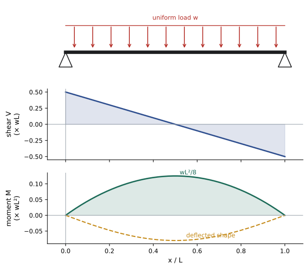
The deflection grows with the fourth power of the span, so doubling the span of a beam multiplies its deflection by 16 under the same load per meter. This strong dependence, visible only through the integration, explains why long-span structures require much deeper sections.

Flow rate from a velocity profile

Fluid flowing through a pipe does not move at the same speed everywhere: friction holds it still at the wall, and it moves fastest at the center. The volume flow rate through the pipe is found by dividing the cross-section into thin rings. A ring of radius \(r\) and width \(dr\) has area \(2\pi r\,dr\), and fluid passes through it at speed \(u(r)\), so:

For slow, steady (laminar) flow of a viscous fluid, the velocity profile is a parabola, \(u(r) = u_{max}\left(1 - \dfrac{r^2}{R^2}\right)\), a result known as Hagen-Poiseuille flow.

The same ring integral gives the momentum and kinetic energy carried by the flow. Because kinetic energy depends on \(u^3\), the energy flux of a non-uniform profile exceeds that computed from the average velocity: for laminar flow by a factor of 2, which fluid mechanics courses include as a kinetic energy correction factor.

Pressure in a fluid at rest and in the atmosphere

In a fluid at rest, the pressure increases with depth because each layer supports the weight of the fluid above. For a thin layer of thickness \(dz\), the balance of forces gives:

with \(z\) measured upward. For a liquid of constant density, integrating gives the familiar \(P = P_0 + \rho g h\) at depth \(h\). In the atmosphere the density is not constant: by the ideal gas law, \(\rho = PM/(RT)\), where \(M\) is the molar mass of air and \(R\) the gas constant. If the temperature is taken as constant, the equation becomes separable (Lesson 5):

Heat conduction through walls and insulation

Fourier's law of heat conduction states that the heat flow rate \(q\) through a material is proportional to the area \(A\) and the temperature gradient: \(q = -kA\,\dfrac{dT}{dx}\), where \(k\) is the thermal conductivity. In steady state the same heat flows through every layer, so \(q\) is constant, and rearranging and integrating across the material gives the temperature drop:

For a flat wall of constant area and conductivity this gives \(q = kA(T_1 - T_2)/L\): the integral is the thermal resistance \(L/(kA)\), and layers in series add their resistances, as Lesson 2 of ELE-470 used for power modules. When the area changes along the path, as it does through the insulation on a pipe, the integral gives a different result.

The same logarithmic resistance governs the heating of buried power cables, whose current rating depends on how easily heat flows outward through the surrounding soil, and the cooling of wires and electronic components. Where the conductivity varies with temperature, as it does for many materials, the integral is written in terms of \(k(T)\,dT\) instead, but the method is the same.

Setting up integrals from elements

Each problem in this lesson followed the same steps, which apply to any new situation:

• Choose an element small enough that the quantity of interest is nearly uniform across it: a slice of beam, a ring of fluid, a cylindrical shell of insulation, a layer of air.
• Write the physical law for the element: equilibrium, mass or energy conservation, Fourier's law, the ideal gas law.
• Express the element's contribution in terms of one variable and its differential.
• Identify the limits and the boundary or initial conditions.
• Integrate, and check the result against units, a limiting case and a known special case.

For example, the pipe insulation result must reduce to the flat-wall formula when the insulation is very thin compared with the pipe radius. With \(r_2 = r_1 + t\) and \(t \ll r_1\), \(\ln(r_2/r_1) \approx t/r_1\) (a Taylor approximation), and the formula becomes \(q \approx k(2\pi r_1 L)(T_1 - T_2)/t\), the flat-wall result with area \(2\pi r_1 L\). Checks like this catch most errors in setting up integrals.