
MATH-300 · Lesson 5 of 5 · 30 min
Numerical integration and ODEs
Integrals and differential equations are the language of engineering, but most of the ones that matter cannot be solved by hand. The discharge of a river is an integral of measured velocities across the channel. The energy in a load cycle is the integral of a recorded power signal. The motion of a vehicle, the temperature of a battery pack and the concentration in a reactor follow differential equations with nonlinear terms that defeat the methods of MATH-201. This chapter covers the methods that compute them anyway: the trapezoidal and Simpson rules, Gauss quadrature, and the Euler and Runge–Kutta methods for ordinary differential equations, along with the idea of stiffness that decides which ODE solver to use.
Numerical integration (quadrature)
The idea is to replace the integrand by an interpolating polynomial (Lesson 4) on each small piece of the interval and integrate that exactly.
The trapezoidal rule
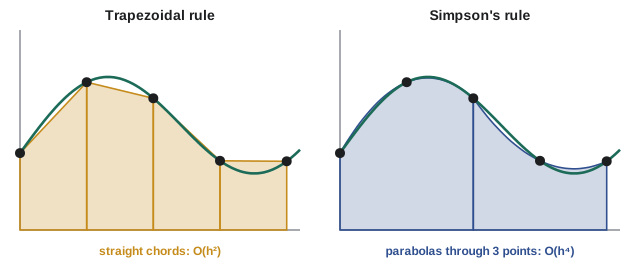
Joining neighboring points with straight lines and adding the areas of the trapezoids gives, for n equal panels of width h,
Its error is about \(\frac{(b - a)h^2}{12}|f''|\): second order, so halving h quarters the error. It is exact for straight lines and works directly on measured data at uneven spacing.
Simpson's rule
Fitting a parabola through each set of three points (an even number of panels) gives Simpson's 1/3 rule:
Its error is about \(\frac{(b - a)h^4}{180}|f^{(4)}|\): fourth order, so halving h divides the error by 16. Surprisingly, it is exact for cubics as well as parabolas.
Worked problem
Comparing the rules
Estimate \(\int_0^\pi \sin x\,dx\) (exactly 2) with n = 4, 8 and 16 panels using both rules.
Show solution
- Trapezoidal: 1.8961 (error 0.104), 1.9742 (0.0258), 1.9936 (0.0064). Each halving of h divides the error by about 4.
- Simpson: 2.00456 (error 0.0046), 2.00027 (0.00027), 2.0000166 (0.0000166). Each halving divides the error by about 16.
Answer: With 16 panels Simpson is accurate to about 8 × 10⁻⁶ relative error, the trapezoidal rule to about 3 × 10⁻³. For smooth integrands, higher order pays off enormously
Worked problem
River discharge from a current-meter survey
A hydrometric crew measures depth and mean velocity at stations 2 m apart across a 16 m wide stream. The unit discharge q = depth × velocity (m²/s) at x = 0, 2, …, 16 m is 0, 0.32, 0.81, 1.25, 1.42, 1.30, 0.94, 0.48, 0. Estimate the discharge \(Q = \int q\,dx\).
Show solution
- Trapezoidal: \(Q = \frac{2}{2}[0 + 2(0.32 + 0.81 + 1.25 + 1.42 + 1.30 + 0.94 + 0.48) + 0] = 13.04\) m³/s.
- Simpson (8 panels): \(Q = \frac{2}{3}[0 + 4(0.32 + 1.25 + 1.30 + 0.48) + 2(0.81 + 1.42 + 0.94) + 0] = 13.16\) m³/s.
Answer: About 13.1 m³/s; the two rules agree within 1%, well inside the uncertainty of the velocity measurements themselves. (Hydrometric practice uses similar panel methods, set out in standards such as ISO 748.)
Richardson extrapolation and adaptive methods
If the error of a rule is known to be proportional to \(h^2\), two estimates with h and h/2 can be combined to cancel the leading error: \(I \approx (4T_{h/2} - T_h)/3\). Applied to the trapezoidal results for sin x with 4 and 8 panels, this gives 2.00027, which is exactly Simpson's rule with 8 panels. Repeating the idea gives Romberg integration. Library routines go further: adaptive quadrature (scipy.integrate.quad, MATLAB integral) estimates the error on each subinterval and refines only where the integrand is difficult, delivering a requested accuracy with as few evaluations as possible.
Gauss quadrature
Newton–Cotes rules (trapezoid, Simpson) use equally spaced points. Gauss quadrature also chooses where to evaluate, picking the points and weights to integrate the highest possible polynomial degree exactly: n points integrate polynomials up to degree 2n − 1 exactly. On [−1, 1] the two-point rule is
Mapped to \([0, \pi]\), two evaluations of sin x give 1.936 and three give 2.0014, better than Simpson with four panels and five evaluations. Gauss quadrature is the standard way finite element programs integrate stiffness matrices over each element, where every evaluation costs real time.
Ordinary differential equations
An initial value problem \(y' = f(t, y)\), \(y(t_0) = y_0\) is solved numerically by stepping forward in time with step h, using the slope f to predict the next value.
Euler's method
The simplest step follows the tangent line:
ENCM-100 used it to simulate a draining tank. It is first order: the global error after reaching a fixed time is proportional to h, so halving the step halves the error and doubles the work. That is too slow for accurate work.
Runge–Kutta methods
Runge–Kutta methods sample the slope at several points within each step and average them. The improved Euler (Heun) method predicts with Euler, then averages the slopes at both ends (second order). The classical fourth-order Runge–Kutta method (RK4) is the most famous:
Four slope evaluations per step buy fourth-order accuracy: halving h divides the error by 16.
Worked problem
A skydiver with air resistance
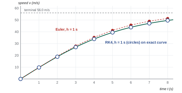
A skydiver of mass 80 kg with drag coefficient c = 0.25 kg/m obeys \(v' = 9.81 - (0.25/80)v^2\), v(0) = 0. The exact solution is \(v = v_t\tanh(9.81t/v_t)\) with terminal speed \(v_t = \sqrt{9.81 \times 80/0.25} = 56.0\) m/s, giving v(4) = 33.875 m/s. Compare Euler, Heun and RK4 at t = 4 s.
Show solution
- Euler, h = 1: v₁ = 0 + 1(9.81) = 9.81; v₂ = 9.81 + 1(9.81 − 0.003125 × 9.81²) = 19.32; … v(4) = 35.33 (error +1.45).
- RK4, first step h = 1: k₁ = 9.810, k₂ = 9.735, k₃ = 9.736, k₄ = 9.514; v₁ = (9.810 + 2(9.735) + 2(9.736) + 9.514)/6 = 9.7109 (exact 9.7110).
- At t = 4 with h = 1: Euler error +1.45; Heun −0.21; RK4 −0.0005.
- With h = 0.5: Euler +0.72 (halved); Heun −0.048 (quartered); RK4 −0.00003 (divided by 16).
Answer: RK4 with four steps of 1 s is accurate to 0.0005 m/s, far better than Euler with 16 steps. The errors scale as h, h² and h⁴, exactly as the orders predict
Systems and higher-order equations
Every method applies unchanged to systems, with y and f as vectors. Higher-order equations are first rewritten as first-order systems. The mass–spring–damper of MATH-201, \(mx'' + cx' + kx = F(t)\), becomes
This is how vehicle suspensions, robot arms, orbits, chemical reactors and power-system transients are simulated.
Stability and stiff equations
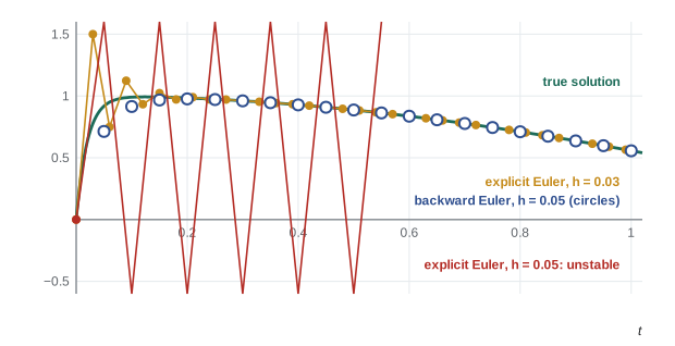
A method can be accurate in principle and still blow up. Applied to the decay equation \(y' = -\lambda y\) (λ > 0), Euler gives \(y_{k+1} = (1 - h\lambda)y_k\), which decays only if \(|1 - h\lambda| < 1\), that is \(h < 2/\lambda\). Larger steps make the numerical solution oscillate and grow without bound, even though the true solution decays to zero.
An equation is stiff when it contains a very fast-decaying component alongside the slow behavior of interest. Explicit methods (Euler, RK4) must then take tiny steps to stay stable, long after the fast component has died away and accuracy no longer needs them. Stiffness is common: chemical kinetics with fast and slow reactions, circuits with very different time constants, and the heat equation on a fine grid.
Worked problem
A stiff equation
Solve \(y' = -50(y - \cos t)\), y(0) = 0, to t = 1. After a quick transient, the solution simply follows about cos t. Try explicit Euler with h = 0.01, 0.03 and 0.05, and the implicit backward Euler method \(y_{k+1} = y_k + hf(t_{k+1}, y_{k+1})\).
Show solution
- Stability limit for explicit Euler: \(h < 2/50 = 0.04\).
- Explicit Euler: h = 0.01 gives 0.557; h = 0.03 gives 0.565; h = 0.05 gives −3325, numerical explosion.
- Backward Euler, solved for \(y_{k+1} = (y_k + 50h\cos t_{k+1})/(1 + 50h)\), gives 0.557 even at h = 0.05, and stays stable for any h.
Answer: The true value is about 0.557. Explicit Euler fails as soon as h exceeds 0.04; the implicit method is stable for any step. Over t = 0 to 10, scipy's explicit RK45 needs 2942 function evaluations; the implicit BDF solver needs 428
Implicit methods must solve an equation (often a nonlinear system, by Newton's method) at every step, so each step costs more, but they can take far larger steps on stiff problems. Library solvers make the choice easy: in scipy.integrate.solve_ivp use RK45 (the default, explicit, adaptive) for ordinary problems and Radau or BDF for stiff ones; MATLAB's equivalents are ode45 and ode15s. If an explicit solver is crawling with tiny steps, suspect stiffness.
import numpy as np
from scipy.integrate import simpson, quad, solve_ivp

x = np.arange(0, 17, 2.0)
q = np.array([0, 0.32, 0.81, 1.25, 1.42, 1.30, 0.94, 0.48, 0])
print(f"discharge (Simpson): {simpson(q, x=x):.2f} m3/s")
print(f"integral of sin on [0, pi]: {quad(np.sin, 0, np.pi)[0]:.10f}")

drag = lambda t, v: 9.81 - (0.25/80)*v**2
sol = solve_ivp(drag, [0, 4], [0.0], rtol=1e-8, atol=1e-10)
print(f"skydiver v(4) = {sol.y[0, -1]:.3f} m/s")

stiff = lambda t, y: -50*(y - np.cos(t))
for method in ["RK45", "BDF"]:
    s = solve_ivp(stiff, [0, 10], [0.0], method=method, rtol=1e-6, atol=1e-9)
    print(f"{method}: y(10) = {s.y[0, -1]:.6f}, function evaluations = {s.nfev}")
Output: discharge (Simpson): 13.16 m3/s; integral of sin on [0, pi]: 2.0000000000; skydiver v(4) = 33.875 m/s; RK45: y(10) = −0.849612, function evaluations = 2942; BDF: y(10) = −0.849612, function evaluations = 428.
Common mistakes
MistakeUsing Simpson's 1/3 rule with an odd number of panels.
InsteadIt needs an even number of panels; use the trapezoidal rule or Simpson's 3/8 rule for the leftover panels.
MistakeAssuming a smaller step is always the answer to inaccuracy.
InsteadA higher-order method or an adaptive library routine is usually far cheaper.
MistakeUsing explicit methods on stiff problems.
InsteadIf steps become tiny, switch to an implicit solver such as BDF or Radau.
MistakeAccepting an ODE solution without checking it.
InsteadTighten the tolerances (or halve h) and confirm the answer does not change; compare with a known special case.
MistakeTrying to apply first-order methods directly to second-order equations.
InsteadRewrite them as first-order systems first.
MistakeIntegrating noisy data with a high-order rule and trusting every digit.
InsteadThe data uncertainty, not the rule, usually limits the accuracy.
Summary and key terms
- The trapezoidal rule (O(h²)) joins points with lines; Simpson's rule (O(h⁴)) uses parabolas and needs an even number of panels.
- Richardson extrapolation and adaptive quadrature improve accuracy automatically; Gauss quadrature chooses optimal points, integrating degree 2n − 1 exactly with n points.
- Euler's method is first order; RK4 uses four slope samples per step for fourth-order accuracy.
- Higher-order ODEs become first-order systems, solved by the same methods.
- Explicit methods are stable only for small enough steps (h < 2/λ for Euler on y′ = −λy).
- Stiff problems need implicit methods (backward Euler, BDF, Radau); library solvers adapt the step to meet error tolerances.
- Quadrature
- Numerical evaluation of a definite integral.
- Trapezoidal rule
- Integration by joining points with straight lines; second order.
- Simpson's rule
- Integration with parabolas through each three points; fourth order.
- Richardson extrapolation
- Combining results at two step sizes to cancel the leading error term.
- Adaptive quadrature
- Refining the integration only where the estimated error is large.
- Gauss quadrature
- Integration using optimally chosen points and weights.
- Initial value problem
- An ODE with the solution specified at the starting time.
- Euler's method
- Stepping along the tangent line; first order.
- Runge–Kutta method
- A one-step ODE method averaging several slope samples per step.
- Stability
- Whether a numerical method keeps errors bounded as it steps forward.
- Stiff equation
- An ODE with widely different time scales, forcing explicit methods to take tiny steps.
- Implicit method
- An ODE method whose update requires solving an equation for the new value.
Practice problems
Work each problem on paper first, then reveal the answer to check.
Use the trapezoidal rule with 2 panels to estimate ∫₀² x² dx (exact 8/3).
Show answer
h = 1: (1/2)[0 + 2(1) + 4] = 3; error 0.333.
Repeat with Simpson's rule.
Show answer
(1/3)[0 + 4(1) + 4] = 8/3: exact, as expected for a quadratic.
A trapezoidal estimate has error 0.08 with 10 panels. Estimate the error with 40 panels.
Show answer
h divided by 4 → error divided by 16: about 0.005.
Trapezoidal estimates of an integral are 5.20 with h and 5.11 with h/2. Give a Richardson-extrapolated value.
Show answer
(4 × 5.11 − 5.20)/3 = 5.08.
Power drawn by a machine (kW) at 0, 10, 20, 30, 40 minutes is 12, 18, 22, 20, 14. Estimate the energy in kWh with Simpson's rule.
Show answer
h = 1/6 h: (1/18)[12 + 4(18) + 2(22) + 4(20) + 14] = 222/18 = 12.3 kWh.
Take two Euler steps with h = 0.1 for y′ = −2y, y(0) = 1. Compare with the exact e^(−0.4).
Show answer
y₁ = 0.8, y₂ = 0.64; exact 0.670; error −0.030.
What is the largest stable Euler step for y′ = −200y?
Show answer
h < 2/200 = 0.01.
Write θ″ + (g/L) sin θ = 0 as a first-order system.
Show answer
y₁ = θ, y₂ = θ′: y₁′ = y₂, y₂′ = −(g/L) sin y₁.
If halving h divides an ODE method's error by about 16, what is its order?
Show answer
Fourth order (2⁴ = 16).
A simulation of fast and slow chemical reactions forces RK45 to take 10⁶ tiny steps. What should you try?
Show answer
The problem is stiff; switch to an implicit solver such as BDF or Radau.
Lesson quiz · 5 questions
Score 60% or more to complete this lesson.
Create a free account to save your progress, take quizzes and earn a certificate.