Capstone: a model honors thesis from question to defense

This final lesson follows Maya's project to its end: the stretch-goal experiment that tested the conductivity dependence of the drag in a new way, the assembly of the thesis from the pieces built over the year, the talk and the defense, and what the examiners said. It then steps back to draw out the general lessons that apply to any honors thesis, whatever the field. The aim is to show the whole cycle of lesson 1 completed once, with the inner loops that made the project better than its first plan, and to give you a concrete picture of what a strong physics honors thesis looks like.

The stretch goal: a cold pipe

By late January the main measurements were finished two weeks ahead of schedule, so Maya turned to hypothesis H4. Comparing copper and aluminum pipes had confirmed that the drag scales with conductivity, but the two pipes were different objects, made by different manufacturers, so the comparison relied on the dimensions and conductivities being measured correctly for each. Changing the temperature of a single pipe changes its conductivity while keeping almost everything else the same: the same geometry, the same slots, the same magnet. Copper's resistivity changes by about 0.39 per 100 per degree near room temperature, so cooling the half-inch type L pipe from 21 degrees to the temperature of a laboratory freezer, about minus 18 degrees, should raise its conductivity by about 18 per 100 and slow the magnet by the same factor.

The experiment needed care. She cooled the pipe overnight in the freezer, carried it to the frame in an insulating sleeve, mounted it quickly, and timed ten drops as fast as the magnet could be retrieved, recording the pipe temperature with a taped thermocouple before and after the set. The pipe warmed by about a degree during the measurements, so she used the mean temperature. Frost was a possible problem: water condensing inside the pipe could add friction, so she flushed the pipe with dry nitrogen gas from the teaching laboratory's supply and checked the inside with a borescope. Thermal contraction shrinks the pipe by about 0.07 per 100 over a 38 degree change, which tightens the gap slightly and increases the drag by roughly 0.3 per 100, a small correction she included. She also remeasured the conductivity of the cold pipe by the four-point method, to confirm the expected change directly rather than relying on the handbook temperature coefficient.

import math
MU0 = 4e-7*math.pi
G = 9.81

def ellip(k):
    """Complete elliptic integrals K(k) and E(k) by the arithmetic-geometric mean."""
    a, b, c = 1.0, math.sqrt(1 - k*k), k
    tot, n = 0.5*c*c, 0
    while abs(c) > 1e-15:
        a, b, c = (a + b)/2, math.sqrt(a*b), (a - b)/2
        n += 1
        tot += 2**(n - 1)*c*c
    K = math.pi/(2*a)
    return K, K*(1 - tot)

def loop_br(I, R, r, z):
    """Radial field of a circular current loop (radius R, current I) at radius r, height z."""
    q = (R + r)**2 + z*z
    K, E = ellip(math.sqrt(4*R*r/q))
    return MU0*I/(2*math.pi)*z/(r*math.sqrt(q))*(-K + (R*R + r*r + z*z)/((R - r)**2 + z*z)*E)

def dipole_br(m, r, z):
    """Radial field of a point dipole m on the axis."""
    return MU0*m/(4*math.pi)*3*r*z/(r*r + z*z)**2.5

def cylinder_br(m, Rm, Lm, r, z, n=24):
    """Uniformly magnetized cylinder treated as n stacked current loops."""
    M = m/(math.pi*Rm*Rm*Lm); dz = Lm/n
    return sum(loop_br(M*dz, Rm, r, z - (-Lm/2 + (i + 0.5)*dz)) for i in range(n))

def drag_k(br, sigma, a, b, nr=6, zmax=0.10, nz=300):
    """Drag coefficient k = sigma * integral of 2 pi r Br^2 over the wall, so that F = k v."""
    tot, h = 0.0, 2*zmax/nz
    for i in range(nr):
        r = a + (i + 0.5)*(b - a)/nr
        s = sum(br(r, -zmax + (j + 0.5)*h)**2 for j in range(nz))*h
        tot += 2*math.pi*r*sigma*s*(b - a)/nr
    return tot

def k_thin(m, sigma, a, b):
    """Point dipole, thin wall at the mean radius: k = 45 mu0^2 m^2 sigma w / (1024 abar^4)."""
    w, abar = b - a, (a + b)/2
    return 45*MU0**2*m*m*sigma*w/(1024*abar**4)

def k_thick(m, sigma, a, b):
    """Point dipole, wall integrated from a to b exactly."""
    return 45*MU0**2*m*m*sigma*(a**-3 - b**-3)/(3*1024)
# Maya's magnet and pipes (lengths in m)
MASS, RM, LM = 12.10e-3, 6.35e-3, 12.70e-3        # magnet mass (kg), radius, length
PIPES = [  # name, inner radius, outer radius, conductivity (S/m)
    ("Cu M 1/2", 7.228e-3, 7.938e-3, 4.95e7),
    ("Cu L 1/2", 6.918e-3, 7.938e-3, 4.95e7),
    ("Cu K 1/2", 6.698e-3, 7.938e-3, 4.95e7),
    ("Al 1/2",   6.698e-3, 7.938e-3, 2.50e7),
    ("Cu L 3/4", 9.973e-3, 11.113e-3, 4.95e7),
]
import random
def drops(name, n=10, seed=2027):
    """Ten transit times (s) over the 0.800 m between the light gates for one pipe."""
    rnd = random.Random(seed + sum(map(ord, name)))
    true_m = 1.62
    for nm, a, b, sig in PIPES:
        if nm == name: break
    vt = 0.975*MASS*G/drag_k(lambda r, z: cylinder_br(true_m, RM, LM, r, z), sig, a, b)
    return [round(0.800/vt*(1 + rnd.gauss(0, 0.010)) + rnd.gauss(0, 0.001), 3) for _ in range(n)]

import math, random
alpha = 0.00393                                   # per degree, copper resistivity near 20 degrees
T_warm, T_cold = 21.4, -17.2
ratio_sigma = (1 + alpha*(T_warm - 20))/(1 + alpha*(T_cold - 20))
contraction = 1 + 0.003                           # drag increase from the slightly smaller gap
predicted = ratio_sigma*contraction               # predicted ratio of cold to warm transit time
warm = drops("Cu L 1/2")
rnd = random.Random(2031)
true_ratio = 1.1813                               # what nature does in this synthetic world
cold = [round(sum(warm)/len(warm)*true_ratio*(1 + rnd.gauss(0, 0.009)) + rnd.gauss(0, 0.001), 3) for _ in range(10)]
def stats(t):
    n = len(t); m = sum(t)/n
    return m, math.sqrt(sum((x - m)**2 for x in t)/(n - 1)/n)
mw, sw = stats(warm); mc, sc = stats(cold)
meas = mc/mw; smeas = meas*math.hypot(sw/mw, sc/mc)
s_pred = predicted*math.hypot(0.005, 0.001)        # temperature reading 0.5 per 100 in the ratio, contraction 0.1
print(f"warm ({T_warm} degrees): mean {mw:.3f} +/- {sw:.3f} s")
print(f"cold ({T_cold} degrees): mean {mc:.3f} +/- {sc:.3f} s")
print(f"measured time ratio  {meas:.4f} +/- {smeas:.4f}")
print(f"predicted time ratio {predicted:.4f} +/- {s_pred:.4f}  (conductivity {ratio_sigma:.4f}, contraction {contraction:.3f})")
print(f"difference: {(meas - predicted)/math.hypot(smeas, s_pred):+.1f} combined standard uncertainties")
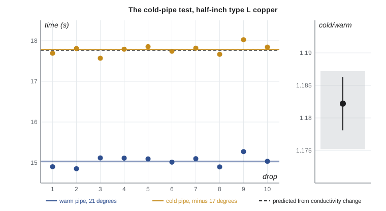
print(f"four-point conductivity ratio measured cold/warm: {1.1771:.4f} (handbook coefficient gives {ratio_sigma:.4f})")

warm (21.4 degrees): mean 15.039 +/- 0.041 s
cold (-17.2 degrees): mean 17.780 +/- 0.039 s
measured time ratio  1.1822 +/- 0.0041
predicted time ratio 1.1812 +/- 0.0060  (conductivity 1.1777, contraction 1.003)
difference: +0.1 combined standard uncertainties
four-point conductivity ratio measured cold/warm: 1.1771 (handbook coefficient gives 1.1777)

The result was a clean confirmation. The magnet took about 18 per 100 longer to cross the cold pipe, and the measured ratio agreed with the prediction from the conductivity change within the combined uncertainty. Her direct four-point measurement of the cold pipe's conductivity agreed with the handbook temperature coefficient to better than 0.1 per 100. The test has a special virtue that she emphasized in the thesis: the predicted ratio does not depend on the dipole moment, the largest uncertainty in the main comparison, because the same magnet falls through the same pipe at both temperatures. It is a test of the conductivity dependence alone, with an uncertainty of under 1 per 100, several times sharper than the absolute comparison.

Assembling the thesis

Maya's thesis was 48 pages plus appendices, and most of it existed in some form before February. Her proposal had become the introduction, revised once the results were in so that its last paragraph stated them. Her reading log and synthesis matrix had become the background chapter, organized by the treatment of the magnet and of the wall rather than by paper. The derivation from lesson 7 became the theory chapter. Her notebook, including the probe-offset story and the two excluded drops, became the methods chapter. The results chapter presented the five pipes, the calibration, the three-model comparison and the cold-pipe test in eight figures and three tables. The discussion interpreted the point-dipole failure, the small finite-magnet residual and the limitations, and listed what a follow-up project should do. Every figure was generated by one script from the read-only raw data, and a single command rebuilt the figures, the results table and the PDF.

import math
MU0 = 4e-7*math.pi
G = 9.81

def ellip(k):
    """Complete elliptic integrals K(k) and E(k) by the arithmetic-geometric mean."""
    a, b, c = 1.0, math.sqrt(1 - k*k), k
    tot, n = 0.5*c*c, 0
    while abs(c) > 1e-15:
        a, b, c = (a + b)/2, math.sqrt(a*b), (a - b)/2
        n += 1
        tot += 2**(n - 1)*c*c
    K = math.pi/(2*a)
    return K, K*(1 - tot)

def loop_br(I, R, r, z):
    """Radial field of a circular current loop (radius R, current I) at radius r, height z."""
    q = (R + r)**2 + z*z
    K, E = ellip(math.sqrt(4*R*r/q))
    return MU0*I/(2*math.pi)*z/(r*math.sqrt(q))*(-K + (R*R + r*r + z*z)/((R - r)**2 + z*z)*E)

def dipole_br(m, r, z):
    """Radial field of a point dipole m on the axis."""
    return MU0*m/(4*math.pi)*3*r*z/(r*r + z*z)**2.5

def cylinder_br(m, Rm, Lm, r, z, n=24):
    """Uniformly magnetized cylinder treated as n stacked current loops."""
    M = m/(math.pi*Rm*Rm*Lm); dz = Lm/n
    return sum(loop_br(M*dz, Rm, r, z - (-Lm/2 + (i + 0.5)*dz)) for i in range(n))

def drag_k(br, sigma, a, b, nr=6, zmax=0.10, nz=300):
    """Drag coefficient k = sigma * integral of 2 pi r Br^2 over the wall, so that F = k v."""
    tot, h = 0.0, 2*zmax/nz
    for i in range(nr):
        r = a + (i + 0.5)*(b - a)/nr
        s = sum(br(r, -zmax + (j + 0.5)*h)**2 for j in range(nz))*h
        tot += 2*math.pi*r*sigma*s*(b - a)/nr
    return tot

def k_thin(m, sigma, a, b):
    """Point dipole, thin wall at the mean radius: k = 45 mu0^2 m^2 sigma w / (1024 abar^4)."""
    w, abar = b - a, (a + b)/2
    return 45*MU0**2*m*m*sigma*w/(1024*abar**4)

def k_thick(m, sigma, a, b):
    """Point dipole, wall integrated from a to b exactly."""
    return 45*MU0**2*m*m*sigma*(a**-3 - b**-3)/(3*1024)
# Maya's magnet and pipes (lengths in m)
MASS, RM, LM = 12.10e-3, 6.35e-3, 12.70e-3        # magnet mass (kg), radius, length
PIPES = [  # name, inner radius, outer radius, conductivity (S/m)
    ("Cu M 1/2", 7.228e-3, 7.938e-3, 4.95e7),
    ("Cu L 1/2", 6.918e-3, 7.938e-3, 4.95e7),
    ("Cu K 1/2", 6.698e-3, 7.938e-3, 4.95e7),
    ("Al 1/2",   6.698e-3, 7.938e-3, 2.50e7),
    ("Cu L 3/4", 9.973e-3, 11.113e-3, 4.95e7),
]
import random
def drops(name, n=10, seed=2027):
    """Ten transit times (s) over the 0.800 m between the light gates for one pipe."""
    rnd = random.Random(seed + sum(map(ord, name)))
    true_m = 1.62
    for nm, a, b, sig in PIPES:
        if nm == name: break
    vt = 0.975*MASS*G/drag_k(lambda r, z: cylinder_br(true_m, RM, LM, r, z), sig, a, b)
    return [round(0.800/vt*(1 + rnd.gauss(0, 0.010)) + rnd.gauss(0, 0.001), 3) for _ in range(n)]

import math, hashlib, json
m0 = 1.62
results = []
for name, a, b, sig in PIPES:
    t = drops(name); mt = sum(t)/len(t)
    v = 0.800/mt
    vf = MASS*G/drag_k(lambda r, z: cylinder_br(m0, RM, LM, r, z), sig, a, b)
    vd = MASS*G/k_thick(m0, sig, a, b)
    results.append({"pipe": name, "v_meas_cm_s": round(v*100, 3), "v_finite_cm_s": round(vf*100, 3),
                    "ratio_finite": round(v/vf, 3), "ratio_dipole": round(v/vd, 3)})
print(f"{'pipe':10s} {'measured':>9s} {'finite':>8s} {'ratio':>7s} {'dipole ratio':>13s}")
for r in results:
    print(f"{r['pipe']:10s} {r['v_meas_cm_s']:9.3f} {r['v_finite_cm_s']:8.3f} {r['ratio_finite']:7.3f} {r['ratio_dipole']:13.3f}")
digest = hashlib.sha256(json.dumps(results, sort_keys=True).encode()).hexdigest()[:16]
print("results-table fingerprint stored with the thesis:", digest)

pipe        measured   finite   ratio  dipole ratio
Cu M 1/2       8.302    8.527   0.974         1.364
Cu L 1/2       5.319    5.458   0.975         1.375
Cu K 1/2       4.063    4.198   0.968         1.367
Al 1/2         8.118    8.312   0.977         1.379
Cu L 3/4      16.578   17.019   0.974         1.173
results-table fingerprint stored with the thesis: 9a7cb77bb2a29bdc

The abstract

Her final abstract, 196 words, read in part: "A magnet falling through a conducting pipe reaches a terminal speed set by eddy-current braking. We test three models of this braking, with no adjustable parameters, against measured terminal speeds in five pipes of copper and aluminum whose inner radii, wall thicknesses and conductivities were measured independently, using a magnet whose dipole moment was calibrated with a Hall probe. Point-dipole models underestimate the measured speeds by 17 to 37 per 100, by an amount that grows as the gap between magnet and wall shrinks. A model that represents the magnet as a uniformly magnetized cylinder predicts the speeds in all five pipes with a single common ratio of 0.973, a 2.7 per 100 offset consistent with the 2.7 per 100 uncertainty of the shared inputs. Cooling one pipe to minus 17 degrees increases the transit time by a factor that agrees with the measured change in conductivity to within 1 per 100." See how the abstract mirrors the thesis: question, method, results with numbers, and a precise statement of agreement.

The talk and the defense

Maya gave her twelve-minute talk at the department's honors day in April, using the plan from lesson 11. The main result came at the start of the results section and again in the conclusion. The first question, from a condensed-matter physicist, was whether the speed could be high enough for the induced currents to distort the field; she had a backup slide estimating the magnetic Reynolds number at about \(10^{-3}\). The second asked whether the 2.7 per 100 residual could come from the moment calibration; she explained that it was about one standard uncertainty, that a 1.3 per 100 error in the moment would remove it, and that the cold-pipe test, which does not depend on the moment, showed the conductivity dependence was right.

In the oral examination the next day, her second reader, Dr. Ingrid Solheim, began with the physics: why does the drag depend on the radial component of the field and not the axial one? Maya answered with the velocity cross product and then drew the field lines of the dipole on the board to show where the radial field is largest. The examiners then went through the uncertainty budget term by term, asked her to derive the beta-function integral without notes, and probed the exclusion of the two early drops, which her notebook entry settled at once. The hardest question was the one in lesson 11's example, about nonuniform magnetization; she acknowledged the assumption, explained which part of the field mattered, and proposed a field map near the magnet's surface as the test. The examiners' report praised the clarity of the model comparison, the honest treatment of the residual and the reproducible analysis, and suggested that the work could become a short paper in a pedagogical journal, which she and Professor Asante began drafting in May.

The classmates' projects

The other four projects ended differently, which is typical. Samir's transit fit recovered the planet's radius ratio within the published uncertainty and showed that the choice of detrending method changed the inclination by more than its quoted error, a modest but genuine methodological result. Jae-won's matched filter found GW150914 at a signal-to-noise ratio close to the published value and recovered a chirp mass consistent with it, though with a larger uncertainty because his template bank was coarser; his thesis was judged excellent for its careful explanation of why. Olivia's muon lifetime came out within two standard uncertainties of the accepted 2.197 microseconds after she discovered and corrected a dead-time effect, the subject of the lesson 9 example. Ravi's critical exponent agreed with the exact 1/8 within his uncertainty, but only after he found that his error bars had been too small by a factor of two because successive samples were correlated, a discovery that became the most interesting chapter of his thesis.

None of the five found anything that will change physics, and none needed to. Each asked a sharp question, built or used a method whose limits they understood, found at least one problem they had not anticipated, and reported the results with honest uncertainties. That is what an honors thesis is for.

What made the project work

Looking back over the year, a few decisions made the difference, and they generalize to any project. The question was sharp from the start: a parameter-free prediction tested against measurements, with an answer that could have gone either way. A rough estimate in the first week showed which inputs mattered, which turned into a calibration plan. The hypotheses were written down with quantitative predictions before the data were taken, which made the comparisons honest and easy to defend. The apparatus, on the critical path, was ordered first. Exact special cases verified the code before it was trusted. The uncertainty budget separated shared from independent errors, which turned a confusing comparison into a clear one. The notebook recorded problems as they happened. Writing started in October. And when the main results came early, the plan had a stretch goal ready, chosen to test the model in a way that avoided its largest uncertainty.

Equally instructive are the things that went wrong and how they were handled. The probe offset cost two weeks and was found because the first calibration gave a moment outside the manufacturer's range and the residuals had a pattern. The two excluded drops were excluded for a documented physical reason and reported. The 2.7 per 100 residual was neither hidden nor overclaimed. Each of these became a strength of the thesis because it was handled openly. Examiners know that research does not go smoothly; what they look for is evidence that the student noticed when it did not, and responded well.