Navigation stacks, map management and evaluation

A SLAM map is only useful when a robot can navigate with it, day after day, while the world changes around it. This lesson moves from algorithms to systems: how a ROS 2 navigation stack uses a map and a localizer to drive a robot safely, how maps are managed across floors, sessions and months of change, and how SLAM and localization quality are measured with standard metrics. Path planning and control algorithms themselves belong to ROB-350; here the focus is on how localization and mapping fit into the navigation system and how to tell whether they are good enough.

The navigation stack

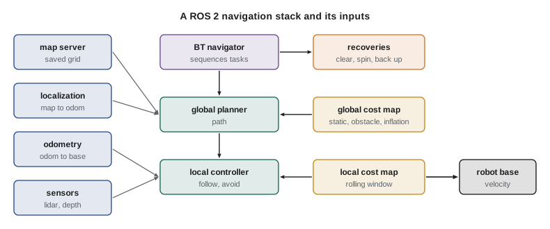
Nav2, the ROS 2 navigation framework (Macenski and colleagues, 2020), is representative of modern navigation stacks. It takes a map, a localization estimate (the transform from map to odom, from AMCL or slam_toolbox in localization mode), odometry (odom to base_link) and sensor data, and drives the robot to goals. Its main parts are a map server, a localizer, a global planner that computes a path through the map, a local controller that follows the path while avoiding obstacles at high rate, cost maps that represent obstacles for both, and a behavior-tree navigator that orchestrates them and handles failures. Each part is a plugin, so planners, controllers and recovery behaviors can be swapped.

Cost maps

A cost map turns the map and live sensor data into a grid of traversal costs. Nav2 builds cost maps from layers. The static layer copies the saved SLAM map. The obstacle layer (or a voxel layer for 3-D sensors) marks obstacles seen by sensors and clears cells that beams pass through, so people, pallets and open doors are represented as they are now. The inflation layer spreads cost outward from every obstacle: cells within the robot's inscribed radius are lethal, and cost then decays exponentially with distance, so planners prefer paths that keep a margin. Keep-out and speed-limit filters add areas that people mark by hand. The global cost map covers the whole map for planning; the local cost map is a small rolling window around the robot, updated at sensor rate, for the controller.

Cost maps are where localization errors become visible as navigation problems. If the localizer is off by 10 cm, the static layer's walls no longer line up with the live obstacle layer's walls, the corridor appears narrower, and the planner may report that the goal is unreachable. A well-tuned stack therefore watches the agreement between the static map and live scans as a health signal.

Behavior trees and recovery

Nav2 sequences navigation with behavior trees, structures of action, condition and control nodes that are easier to extend and reason about than state machines. A typical tree computes a path, follows it, and replans at a fixed rate or when the path becomes blocked. When something fails, recovery behaviors run in a configured order: clear the cost maps (removing stale obstacles), spin in place (letting the sensors refresh and, if localization is uncertain, giving the particle filter new views), back up, or wait for a dynamic obstacle to move. If all recoveries fail, the navigator aborts and reports the failure to a higher-level task manager or fleet manager. Many localization problems surface as repeated recoveries, so recovery logs are a valuable diagnostic.

<!-- Excerpt of a Nav2 BT: navigate with replanning and recoveries -->
<root BTCPP_format="4" main_tree_to_execute="MainTree">
  <BehaviorTree ID="MainTree">
    <RecoveryNode number_of_retries="6" name="NavigateRecovery">
      <PipelineSequence name="NavigateWithReplanning">
        <RateController hz="1.0">
          <ComputePathToPose goal="{goal}" path="{path}" planner_id="GridBased"/>
        </RateController>
        <FollowPath path="{path}" controller_id="FollowPath"/>
      </PipelineSequence>
      <ReactiveFallback name="RecoveryFallback">
        <GoalUpdated/>
        <RoundRobin name="RecoveryActions">
          <ClearEntireCostmap service_name="local_costmap/clear_entirely_local_costmap"/>
          <Spin spin_dist="1.57"/>
          <Wait wait_duration="5"/>
          <BackUp backup_dist="0.30" backup_speed="0.05"/>
        </RoundRobin>
      </ReactiveFallback>
    </RecoveryNode>
  </BehaviorTree>
</root>

Map management

A deployed map has a life cycle. It is created during commissioning by a planned mapping run, cleaned (removing people and temporary objects captured during mapping, straightening walls if needed), annotated with keep-out zones, speed zones, docking stations and named goals, validated, and then versioned. Changes to the environment, such as new racking or a moved wall, require updating or re-mapping. For fleets, one master map is shared by all robots, so updates must be distributed consistently, and each robot's localizer must load the same version.

Large and multi-floor sites need more structure. Multi-floor operation keeps one map per floor and switches maps when the robot rides a lift, re-initializing localization at a known pose by the lift door. Very large sites split maps into tiles or submaps loaded as the robot moves. Outdoor robots often combine a local SLAM map with GNSS for global position, aligning the map frame to a geographic frame such as UTM.

Lifelong mapping addresses gradual change. Instead of freezing the map, the robot keeps updating it: slam_toolbox's lifelong mode adds new scans to the saved pose graph on later runs and removes old nodes whose scans no longer match, so the map tracks the environment while its size stays bounded. Research systems maintain multiple map versions per place (for example, door open and door closed) or model the probability that each part of the map changes, using frequency or time-of-day patterns. Dynamic objects should not be written into the long-term map at all; filtering detected people and vehicles before mapping keeps it clean.

Evaluating SLAM and localization

Claims that a SLAM system is accurate need numbers, and the community has standard metrics, popularized by the TUM RGB-D benchmark (Sturm and colleagues, 2012) and the KITTI benchmark (Geiger and colleagues, 2012). Both compare an estimated trajectory with a ground-truth trajectory from a more accurate system, such as a motion-capture system indoors or RTK GNSS with an inertial navigation system outdoors.

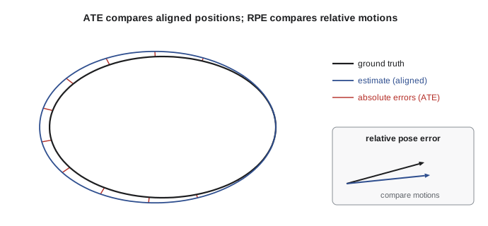
The absolute trajectory error (ATE) measures global consistency. First, the estimated trajectory is aligned to the ground truth with the best rigid transform (or a similarity transform for monocular systems), computed in closed form by the Umeyama method, which is the same SVD alignment as ICP with known correspondences. Then the error is the root-mean-square of the position differences:

The relative pose error (RPE) measures local accuracy, or drift: for each pair of poses a fixed interval apart (in time or distance), compare the estimated relative motion with the true relative motion. RPE is independent of where errors happened along the trajectory, which makes it the right metric for odometry; KITTI reports it as average translational error in percent over segments of 100 m to 800 m, and rotational error in degrees per meter. ATE is the right metric for the global map, because a single uncorrected loop can make ATE large even if RPE is small. The evo and rpg_trajectory_evaluation tools compute both.

import numpy as np
rng = np.random.default_rng(9)
t = np.linspace(0, 2 * np.pi, 200)
gt = np.column_stack([10 * np.cos(t), 6 * np.sin(t)])               # ground-truth loop
th = np.radians(5)
R0 = np.array([[np.cos(th), -np.sin(th)], [np.sin(th), np.cos(th)]])
drift = np.column_stack([np.linspace(0, 0.6, 200), np.linspace(0, -0.3, 200)])
est = (gt + drift + rng.normal(0, 0.05, gt.shape)) @ R0.T + [3.0, -2.0]   # rotated, shifted frame
def umeyama(src, dst):                                                # rigid alignment (no scale)
    ms, md = src.mean(0), dst.mean(0)
    U, S, Vt = np.linalg.svd((dst - md).T @ (src - ms))
    D = np.diag([1, np.sign(np.linalg.det(U @ Vt))])
    R = U @ D @ Vt; return R, md - R @ ms
R, tr = umeyama(est, gt)
aligned = est @ R.T + tr
ate = np.sqrt(np.mean(np.sum((aligned - gt) ** 2, 1)))
d = 20                                                                 # RPE over 20-pose intervals
rel_gt = gt[d:] - gt[:-d]; rel_est = aligned[d:] - aligned[:-d]
rpe = np.sqrt(np.mean(np.sum((rel_est - rel_gt) ** 2, 1)))
seg = np.mean(np.linalg.norm(rel_gt, axis=1))
print("ATE RMSE after alignment: %.3f m" % ate)
print("RPE RMSE over %d-pose segments (mean length %.2f m): %.3f m (%.2f %%)" % (d, seg, rpe, 100 * rpe / seg))
print("unaligned mean error would be: %.2f m" % np.mean(np.linalg.norm(est - gt, axis=1)))

ATE RMSE after alignment: 0.200 m
RPE RMSE over 20-pose segments (mean length 5.18 m): 0.129 m (2.48 %)
unaligned mean error would be: 3.97 m

Safety standards for mobile robots

Localization and mapping are not safety functions in themselves; standards require that collision avoidance and speed limits be enforced by safety-rated systems, typically safety laser scanners with configurable protective fields, that do not depend on SLAM being right.

In the US, ANSI/A3 R15.08-1 (2020) sets safety requirements for industrial mobile robots and R15.08-2 (2023) covers their integration into systems and applications, with ISO 3691-4 widely used for driverless industrial trucks and R15.06 for robot arms on mobile platforms. OSHA has no specific mobile robot standard, but its general duty clause and machinery rules apply, and the standards are used to show that hazards have been addressed.

Both countries' frameworks expect a risk assessment of the application, protective fields sized for the robot's stopping distance at each speed, and speed limits in shared areas, all independent of the navigation stack's software.