Second-order linear equations

Newton's second law involves acceleration, a second derivative, so the equations of mechanics are second order. So are the equations for electrical circuits with inductance, the deflection of beams, and the vibration of structures. Fortunately, the most important of these are linear with constant coefficients, and for that class there is a complete and elegant method: guess an exponential, solve a quadratic, and read off the behaviour.

This chapter develops that method for homogeneous equations (three cases, depending on the roots), shows how to fit initial conditions, then handles forcing terms with the method of undetermined coefficients, including the special case that leads to resonance. It finishes with a boundary value problem that every civil and mechanical engineer uses: the deflection of a uniformly loaded beam.

The standard form and superposition

A second-order linear equation with constant coefficients has the form

If \(f(t) = 0\) the equation is homogeneous; otherwise \(f\) is the forcing term. Linearity gives the key property, the principle of superposition: if \(y_1\) and \(y_2\) solve the homogeneous equation, so does any combination \(C_1y_1 + C_2y_2\). A second-order equation needs two independent solutions, and its general solution has two constants, fixed by two conditions such as the initial position and velocity.

For the nonhomogeneous equation, the general solution is the sum of the homogeneous solution and any one particular solution:

Physically, \(y_h\) is the system's natural (free) response, which depends on how it started and usually dies away; \(y_p\) is the response forced by the input.

Homogeneous equations: the characteristic equation

Try \(y = e^{rt}\). Then \(y' = re^{rt}\) and \(y'' = r^2e^{rt}\), and substituting into \(ay'' + by' + cy = 0\) gives \(e^{rt}(ar^2 + br + c) = 0\). Since \(e^{rt}\) is never zero, r must satisfy the characteristic equation

The discriminant \(b^2 - 4ac\) decides the form of the solution.

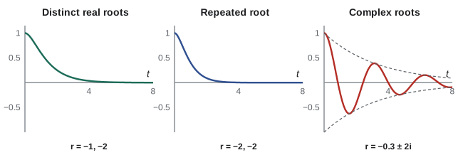
Case 1: two distinct real roots

If \(b^2 > 4ac\), there are two real roots \(r_1 \ne r_2\), and

Case 2: a repeated root

If \(b^2 = 4ac\), the single root is \(r = -b/(2a)\), and the second independent solution is \(te^{rt}\):

Case 3: complex roots

If \(b^2 < 4ac\), the roots are complex: \(r = \alpha \pm i\beta\), with \(\alpha = -b/(2a)\) and \(\beta = \sqrt{4ac - b^2}/(2a)\). Using Euler's formula \(e^{i\beta t} = \cos\beta t + i\sin\beta t\), the real solutions are

This is an oscillation at angular frequency \(\beta\) inside an envelope \(e^{\alpha t}\) that decays when \(\alpha < 0\). It is the mathematics of every vibrating structure and every tuned circuit.

Nonhomogeneous equations: undetermined coefficients

When the forcing \(f(t)\) is a polynomial, an exponential, a sine or cosine, or a product of these, the particular solution has the same form with unknown coefficients. Substitute and match terms.

• Constant or polynomial of degree n: try a polynomial of degree n.
• \(e^{kt}\): try \(Ae^{kt}\).
• \(\sin\omega t\) or \(\cos\omega t\): try \(A\cos\omega t + B\sin\omega t\) (both terms, even if only one appears in f).

That split, transient plus steady state, is how engineers think about any forced linear system. After a few time constants, only the forced response matters, which is why the steady-state amplitude is the quantity checked against limits in vibration and AC circuit design.

The modification rule and resonance

If the trial form already solves the homogeneous equation, it cannot be a particular solution: substituting gives zero. Multiply the trial by t (by \(t^2\) if needed).

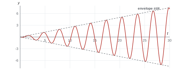
Real structures always have some damping, which limits the growth, but lightly damped systems can still reach dangerous amplitudes at resonance. Lesson 3 quantifies this.

Variation of parameters

When the forcing is not of the simple forms above (for example \(\tan t\) or \(1/t\)), a more general method, variation of parameters, builds \(y_p\) from the homogeneous solutions using integrals. In practice, engineers handle arbitrary forcing with Laplace transforms (Lesson 4) or numerical solution, so we note the method and move on.

A boundary value problem: beam deflection

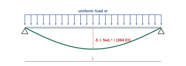
Not every second-order problem starts from initial conditions. For a beam, the conditions are at the two ends: a boundary value problem. For small deflections, the beam's deflection \(v(x)\) (positive upward) satisfies

where M is the bending moment (positive when sagging), E the modulus of elasticity and I the second moment of area (MATH-209, Lesson 3). For a simply supported beam with a uniform load w over a span L, statics (ENGG-130) gives \(M(x) = \tfrac{w}{2}(Lx - x^2)\).

This formula, \(5wL^4/384EI\), is among the most used in structural engineering. Notice what the differential equation reveals: deflection grows with the fourth power of span. Doubling the span of a floor makes it sixteen times more flexible, which is why long spans need deep beams.