
MATH-209 · Lesson 11 of 12 · 27 min
Vector calculus in electromagnetism
Lesson 8 met Gauss's law and Ampère's law as applications of the divergence and Stokes theorems. Together with two more laws, they make up Maxwell's equations, which govern every electrical machine, circuit, antenna, cable and optical fibre. This lesson assembles the four equations in integral form, converts them to differential form using the theorems of Lesson 8, and uses the tools of Lessons 9 and 10 to solve engineering problems with them: the potential and capacitance of a coaxial cable and the best proportions for it, shielding by a conducting enclosure, the voltage induced in a generator coil, and a numerical solution of Laplace's equation. It ends with the most striking consequence of all: combining the equations predicts electromagnetic waves travelling at the speed of light.
Maxwell's equations
In integral form, for any closed surface S enclosing a volume, and any surface Σ with boundary curve C:
| Law | Integral form | Differential form |
|---|---|---|
| Gauss (electric) | \(\oiint_S \mathbf{E} \cdot \mathbf{n}\,dS = Q_{enc}/\varepsilon_0\) | \(\nabla \cdot \mathbf{E} = \rho/\varepsilon_0\) |
| Gauss (magnetic) | \(\oiint_S \mathbf{B} \cdot \mathbf{n}\,dS = 0\) | \(\nabla \cdot \mathbf{B} = 0\) |
| Faraday | \(\oint_C \mathbf{E} \cdot d\mathbf{r} = -\dfrac{d}{dt}\iint_\Sigma \mathbf{B} \cdot \mathbf{n}\,dS\) | \(\nabla \times \mathbf{E} = -\dfrac{\partial \mathbf{B}}{\partial t}\) |
| Ampère-Maxwell | \(\oint_C \mathbf{B} \cdot d\mathbf{r} = \mu_0 I_{enc} + \mu_0\varepsilon_0\dfrac{d}{dt}\iint_\Sigma \mathbf{E} \cdot \mathbf{n}\,dS\) | \(\nabla \times \mathbf{B} = \mu_0\mathbf{J} + \mu_0\varepsilon_0\dfrac{\partial \mathbf{E}}{\partial t}\) |
The conversion is the same each time. For Gauss's law, the divergence theorem turns the flux through S into the integral of \(\nabla \cdot \mathbf{E}\) over the volume, and the enclosed charge is the integral of the charge density ρ; since the equality holds for every volume, the integrands are equal. For Faraday's law, Stokes' theorem turns the circulation around C into the flux of the curl through Σ; since this holds for every surface, the curl equals \(-\partial\mathbf{B}/\partial t\). The integral forms are best for symmetric problems and for understanding; the differential forms hold at every point and are what numerical field solvers discretize.
In words: electric field lines start and end on charges; magnetic field lines never end; a changing magnetic field induces a circulating electric field (the principle of transformers and generators); and currents and changing electric fields create circulating magnetic fields. Maxwell's addition, the displacement-current term \(\mu_0\varepsilon_0\,\partial\mathbf{E}/\partial t\), is needed for consistency: taking the divergence of the Ampère-Maxwell equation, the left side vanishes (div curl = 0, Lesson 9), and the right side then reproduces the continuity equation for charge, \(\partial\rho/\partial t + \nabla \cdot \mathbf{J} = 0\), the same form as conservation of mass in Lesson 10.
Electrostatics and the potential
When nothing changes with time, Faraday's law gives \(\nabla \times \mathbf{E} = \mathbf{0}\), so the electric field has a scalar potential: \(\mathbf{E} = -\nabla V\), where V is the voltage. Substituting into Gauss's law gives Poisson's equation, and in charge-free regions Laplace's equation:
In a material, the permittivity \(\varepsilon = \varepsilon_r\varepsilon_0\) replaces \(\varepsilon_0\). So electrostatics, steady heat conduction, ideal flow and groundwater seepage all reduce to Laplace's equation, and a solution found in one field can be reinterpreted in the others. Engineers once built conducting-paper and electrolytic-tank analogues to solve seepage and heat flow problems by measuring voltages.
Worked problem
A coaxial cable
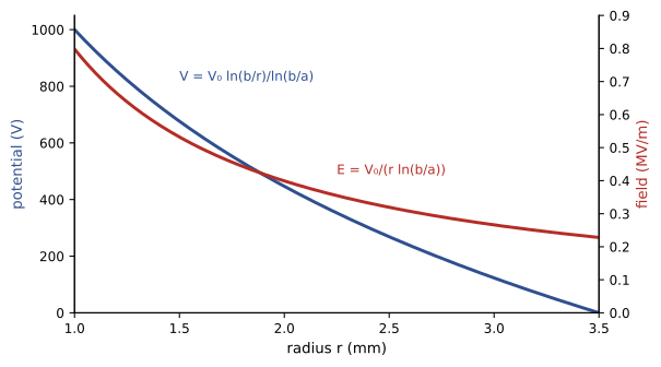
A coaxial cable has an inner conductor of radius a = 1.0 mm at voltage \(V_0\), an outer conductor of radius b = 3.5 mm at 0 V, and polyethylene insulation with \(\varepsilon_r = 2.25\). Find the potential and field in the insulation, the capacitance per metre and the maximum field for \(V_0\) = 1.0 kV.
Show solution
- Laplace's equation in cylindrical coordinates with V depending only on r (Lesson 9): \(V = A\ln r + B\).
- Boundary conditions give \(V = V_0\,\dfrac{\ln(b/r)}{\ln(b/a)}\), and \(E = -\dfrac{dV}{dr} = \dfrac{V_0}{r\ln(b/a)}\).
- Gauss's law gives the charge per metre on the inner conductor, \(q' = 2\pi\varepsilon aE(a) = 2\pi\varepsilon V_0/\ln(b/a)\), so \(C' = 2\pi\varepsilon/\ln(b/a)\).
- \(C' = 2\pi \times 8.854 \times 10^{-12} \times 2.25/\ln 3.5 = 99.9\) pF/m.
- Maximum field at r = a: \(E = 1000/(0.001 \times 1.253) = 0.80\) MV/m.
Answer: V = V₀ ln(b/r)/ln(b/a), E = V₀/(r ln(b/a)), C′ ≈ 100 pF/m, and a peak field of 0.80 MV/m at the surface of the inner conductor, well below the breakdown strength of polyethylene (tens of MV/m). The field is strongest at the inner conductor, so that is where insulation fails first.
Choosing the best proportions
For a given outer radius b and an insulation that breaks down at field \(E_{max}\), what inner radius allows the highest voltage? From the field formula, \(V_0 = E_{max}\,a\ln(b/a)\). Maximizing over a (one-variable optimization) gives \(\ln(b/a) = 1\), so \(b/a = e \approx 2.72\). A smaller inner conductor concentrates the field too much; a larger one leaves too little insulation. High-voltage cable designers use this result, adjusted for other constraints such as conductor resistance.
Shielding and uniqueness
Laplace's equation has a uniqueness property: in a region, the solution is completely determined by its values on the boundary. Combined with the maximum principle for harmonic functions (Lesson 9), this explains electrostatic shielding. Inside a hollow, charge-free region enclosed by a conductor, the conductor surface has a single potential \(V_c\). The constant function \(V = V_c\) satisfies Laplace's equation and the boundary condition, so by uniqueness it is the solution: the field inside is exactly zero, whatever charges are outside. This is the Faraday cage, used to shield sensitive instruments, MRI rooms and the electronics in aircraft struck by lightning. Uniqueness also justifies the method of images, in which a problem with a conducting plane is solved by inventing a mirror-image charge: if a guessed solution satisfies the equation and the boundary conditions, it is the solution.
Numerical solution of Laplace's equation
For shapes without symmetry, Laplace's equation is solved numerically. On a square grid with spacing h, the second derivatives are replaced by differences, and \(\nabla^2V = 0\) becomes the statement that each interior value is the average of its four neighbours, the discrete version of the mean-value property. The simplest solution method sweeps the grid repeatedly, replacing each value by the average of its neighbours, until nothing changes (Gauss-Seidel iteration, MATH-125). Over-relaxation, overshooting each update by a factor ω between 1 and 2, speeds this up dramatically.
import numpy as np

def solve(n, omega, tol=1e-6):
    V = np.zeros((n, n))
    V[0, :] = 100.0                 # lid at 100 V; other sides stay at 0 V
    for sweep in range(1, 100001):
        change = 0.0
        for i in range(1, n - 1):
            for j in range(1, n - 1):
                avg = 0.25 * (V[i + 1, j] + V[i - 1, j] + V[i, j + 1] + V[i, j - 1])
                new = V[i, j] + omega * (avg - V[i, j])
                change = max(change, abs(new - V[i, j]))
                V[i, j] = new
        if change < tol:
            return V, sweep

n = 41
omega_opt = 2 / (1 + np.sin(np.pi / (n - 1)))
for omega in [1.0, omega_opt]:
    V, sweeps = solve(n, omega)
print(f"omega = {omega:.3f}: {sweeps:5d} sweeps, potential at the middle {V[n // 2, n // 2]:.3f} V")omega = 1.000: 2005 sweeps, potential at the middle 25.000 V omega = 1.854: 121 sweeps, potential at the middle 25.000 V
The centre value converges to 25 V, a quarter of the lid voltage, as the symmetry argument predicts (four boxes, each with one side at 100 V, add up to a box entirely at 100 V). Over-relaxation reduces the number of sweeps by more than a factor of ten. Commercial finite element programs use more sophisticated grids and solvers, but the principle is the same.
Magnetic fields and induction
Since \(\nabla \cdot \mathbf{B} = 0\), the magnetic field has a vector potential, \(\mathbf{B} = \nabla \times \mathbf{A}\) (Lesson 9). For steady currents with symmetry, Ampère's law gives the field directly; for a long straight wire it is \(B = \mu_0I/(2\pi r)\), circling the wire, the same 1/r form as the free vortex of Lesson 9, with all the "vorticity" concentrated in the current.
Faraday's law in integral form says that the voltage (EMF) around a loop equals minus the rate of change of magnetic flux through it. For a coil of N turns and area A rotating at angular speed ω in a uniform field B, the flux through each turn is \(BA\cos\omega t\), so
Worked problem
A simple alternator
A coil of 100 turns with area 0.010 m² rotates at 60 revolutions per second in a field of 0.50 T. Find the peak and RMS voltage.
Show solution
- \(\omega = 2\pi \times 60 = 377\) rad/s.
- Peak: \(NBA\omega = 100 \times 0.50 \times 0.010 \times 377 = 189\) V.
- RMS: \(189/\sqrt{2} = 133\) V.
Answer: A peak of 189 V and an RMS value of 133 V at 60 Hz. Doubling the speed doubles both the voltage and the frequency, which is why generators connected to the grid must run at a fixed synchronous speed.
Electromagnetic waves
In empty space (\(\rho = 0\), \(\mathbf{J} = \mathbf{0}\)), take the curl of Faraday's law and use the identity \(\nabla \times (\nabla \times \mathbf{E}) = \nabla(\nabla \cdot \mathbf{E}) - \nabla^2\mathbf{E}\) from Lesson 9. Since \(\nabla \cdot \mathbf{E} = 0\):
So each component of E satisfies the wave equation (MATH-201) with wave speed
When Maxwell found that this speed, computed from laboratory measurements of electric and magnetic forces, equalled the measured speed of light, he concluded that light is an electromagnetic wave. A plane wave has E and B perpendicular to each other and to the direction of travel, with \(|\mathbf{B}| = |\mathbf{E}|/c\). In a material, ε and μ replace their vacuum values and the wave slows down: in polyethylene, with \(\varepsilon_r = 2.25\), signals travel at c/1.5, two-thirds of the speed of light, which sets the delay in coaxial cables.
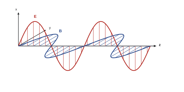
The energy carried by the wave is described by the Poynting vector \(\mathbf{S} = \mathbf{E} \times \mathbf{B}/\mu_0\), whose flux through a surface is the power crossing it. Applying the divergence theorem to the energy stored in the fields gives a conservation law of exactly the form seen for heat and mass: the rate of decrease of field energy in a region equals the power flowing out through its surface plus the power delivered to charges inside. The same pattern, a conserved quantity, a flux and the divergence theorem, has now appeared for heat, mass, momentum, charge and electromagnetic energy.
Common mistakes
MistakeForgetting the displacement current in the Ampère-Maxwell law.
InsteadWithout μ₀ε₀∂E/∂t the equations violate conservation of charge and predict no waves.
MistakeWriting E = ∇V.
InsteadE = −∇V: the field points from high to low potential.
MistakeAssuming the field in a coaxial cable is uniform.
InsteadIt varies as 1/r and is strongest at the inner conductor.
MistakeUsing ε₀ inside a dielectric.
InsteadUse ε = εᵣε₀ for the insulation.
MistakeExpecting the field inside a closed conductor to depend on outside charges.
InsteadBy uniqueness, the field in an empty conducting enclosure is zero.
Summary and key terms
- Maxwell's equations relate the divergence and curl of E and B to charges, currents and changing fields.
- The divergence and Stokes theorems convert between integral and differential forms.
- In electrostatics E = −∇V and V satisfies Poisson's or Laplace's equation.
- A coaxial cable has V ∝ ln(b/r), E ∝ 1/r and C′ = 2πε/ln(b/a); b/a = e maximizes the voltage rating.
- Uniqueness of Laplace solutions explains shielding by conducting enclosures and the method of images.
- Faraday's law gives a generator EMF of NBAω sin ωt.
- Maxwell's equations predict waves travelling at c = 1/√(μ₀ε₀), the speed of light.
- Maxwell's equations
- The four laws governing electric and magnetic fields.
- Displacement current
- The term ε₀∂E/∂t that completes Ampère's law.
- Electric potential
- A scalar V with E = −∇V.
- Poisson's equation
- ∇²V = −ρ/ε, relating potential to charge density.
- Permittivity
- ε = εᵣε₀, a material's response to an electric field.
- Capacitance per unit length
- Charge per metre divided by voltage for a cable or line.
- Faraday cage
- A conducting enclosure inside which the static electric field is zero.
- EMF
- The induced voltage around a loop, equal to minus the rate of change of magnetic flux.
- Over-relaxation
- Accelerating an iterative solver by overshooting each update.
- Poynting vector
- S = E × B/μ₀, the power flow per unit area of an electromagnetic field.
Practice problems
Work each problem on paper first, then reveal the answer to check.
Find \(\nabla \cdot \mathbf{E}\) for \(\mathbf{E} = (2x, 3y, -z)\) and the charge density.
Show answer
4; ρ = 4ε₀.
Find E from \(V = 5x^2 - 3y\).
Show answer
E = (−10x, 3, 0).
Find the capacitance per metre of an air-filled coax with b/a = e.
Show answer
2πε₀ = 55.6 pF/m.
A coax has a = 0.5 mm, b = 2.5 mm and V₀ = 500 V. Find E at the inner conductor.
Show answer
500/(0.0005 × ln 5) = 0.62 MV/m.
With b = 10 mm and E_max = 20 MV/m, what is the highest voltage rating and the best a?
Show answer
a = b/e = 3.68 mm; V = E_max a = 73.6 kV.
Find the magnetic field 50 mm from a wire carrying 200 A.
Show answer
μ₀I/(2πr) = 0.80 mT.
A 50-turn coil of area 0.02 m² spins at 3000 rpm in 0.4 T. Find the peak EMF.
Show answer
ω = 314 rad/s; 50 × 0.4 × 0.02 × 314 = 126 V.
Show that the divergence of the Ampère-Maxwell law gives conservation of charge.
Show answer
0 = μ₀∇ · J + μ₀ε₀∂(∇ · E)/∂t = μ₀(∇ · J + ∂ρ/∂t).
At what speed do signals travel in a cable with εᵣ = 4?
Show answer
c/2 = 1.5 × 10⁸ m/s.
How long does a signal take to travel 100 m of polyethylene coax?
Show answer
100/(2 × 10⁸) = 0.5 µs.
Lesson quiz · 5 questions
Score 60% or more to complete this lesson.
Create a free account to save your progress, take quizzes and earn a certificate.