
MATH-300 · Lesson 9 of 12 · 30 min
Boundary value problems
Lessons 7 and 8 solved initial value problems, where everything is known at the start and the solver marches forward. Many engineering problems instead fix conditions at two ends: the temperature at the base of a fin and the heat flow at its tip, the supports at both ends of a beam, the launch point and the target of a projectile, the concentrations at the two faces of a membrane. These boundary value problems (BVPs) cannot be marched directly, because the missing starting values are unknown, and MATH-201 showed that they may have one solution, several or none. This lesson develops the two main numerical approaches. The shooting method turns a BVP into a root-finding problem (Lesson 2) wrapped around an IVP solver. Finite difference methods replace derivatives by differences on a grid and solve a system of equations (Lesson 3), using Newton's method when the problem is nonlinear. The lesson also shows how a BVP with an unknown parameter becomes a matrix eigenvalue problem (Lesson 4), the numerical route to buckling loads and mode shapes.
The shooting method
For a second-order BVP such as \(y'' = f(x, y, y')\) with \(y(a) = \alpha\) and \(y(b) = \beta\), guess the missing initial slope s, solve the IVP from a to b with \(y(a) = \alpha\), \(y'(a) = s\), and see how far \(y(b)\) misses β. The miss distance \(F(s) = y(b; s) - \beta\) is a function of one variable, and the BVP is solved when \(F(s) = 0\). Any root finder will do: bisection if two guesses bracket the target, the secant method otherwise. For a linear equation, F is linear in s, so two shots and one interpolation give the exact answer.
Shooting is intuitive and uses accurate adaptive IVP solvers, and it handles nonlinear problems naturally. It has two weaknesses. If the IVP is sensitive, with solutions that grow rapidly (as in some problems with exponential behaviour over long intervals), small changes in s produce enormous changes at b and the root finder struggles; multiple shooting, which breaks the interval into pieces joined by matching conditions, cures this. And it does not extend easily to problems in two or three dimensions.
Worked problem
Aiming a projectile
A ball is thrown at 30 m/s with quadratic air drag (drag acceleration \(kv^2\) with k = 0.01 m⁻¹). At what launch angle does it land 45 m away?
Show solution
- The equations of motion are an IVP in the launch angle; the condition "lands at 45 m" is the second boundary condition.
- Define F(θ) = landing distance − 45, computing the landing point with an event function (Lesson 8).
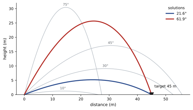
- Shots at several angles show that F changes sign between 10° and 30°, and again between 45° and 75°, so bisection or Brent's method can find both roots.
Answer: Two solutions, about 21.6° (a flat throw) and 61.9° (a lob), as the code shows. With drag the maximum range is about 56 m, reached near 40° rather than 45°, so a target beyond 56 m has no solution: a BVP need not be solvable.
import numpy as np
from scipy.integrate import solve_ivp
from scipy.optimize import brentq

# Ball launched at 30 m/s with quadratic drag; find the launch angle that lands 45 m away
g, k, v0, target = 9.81, 0.01, 30.0, 45.0     # k = drag constant per unit mass (1/m)

def rhs(t, s):
    x, y, vx, vy = s
    v = np.hypot(vx, vy)
    return [vx, vy, -k * v * vx, -g - k * v * vy]

def landing(t, s):
    return s[1]
landing.terminal, landing.direction = True, -1

def miss(angle_deg):
    a = np.radians(angle_deg)
    sol = solve_ivp(rhs, [0, 20], [0, 0, v0 * np.cos(a), v0 * np.sin(a)], events=landing,
                    rtol=1e-9, atol=1e-9)
    return sol.y_events[0][0][0] - target

for a in [10, 20, 30, 45, 60, 75]:
    print(f"angle {a:2d} deg: lands {miss(a) + target:6.2f} m")
low = brentq(miss, 5, 38)
high = brentq(miss, 42, 85)
print(f"Shooting solutions: {low:.3f} deg (flat) and {high:.3f} deg (lob)")angle 10 deg: lands 26.13 m angle 20 deg: lands 42.96 m angle 30 deg: lands 52.61 m angle 45 deg: lands 55.78 m angle 60 deg: lands 46.90 m angle 75 deg: lands 27.36 m Shooting solutions: 21.645 deg (flat) and 61.882 deg (lob)
Finite difference methods
The finite difference method treats the whole interval at once. Divide \([a, b]\) into N intervals of width h, with unknown values \(y_i\) at the grid points, and replace each derivative by a centred difference (Lesson 1):
Both approximations have error proportional to \(h^2\). Writing the differential equation at every interior point gives one equation per unknown. For a linear second-order equation, each equation involves only three neighbouring unknowns, so the system is tridiagonal and can be solved in \(O(N)\) operations (the Thomas algorithm, or scipy.linalg.solve_banded), even for millions of points.
Boundary conditions enter in two ways. A fixed value (a Dirichlet condition, such as a given base temperature) simply replaces an unknown with a known number, moved to the right side. A derivative condition (a Neumann condition, such as an insulated tip with zero heat flow) is handled with a ghost point beyond the boundary: the centred condition \((y_{N+1} - y_{N-1})/(2h) = 0\) gives \(y_{N+1} = y_{N-1}\), which is substituted into the equation at the boundary point, keeping second-order accuracy.
Worked problem
A cooling fin by finite differences
Set up the finite difference equations for the fin equation \(\theta'' - m^2\theta = 0\) with \(\theta(0) = 1\) and an insulated tip \(\theta'(L) = 0\).
Show solution
- Interior points: \(\theta_{i-1} - (2 + m^2h^2)\theta_i + \theta_{i+1} = 0\) for i = 1, …, N − 1, with \(\theta_0 = 1\) moved to the right side of the first equation.
- Tip, using the ghost point \(\theta_{N+1} = \theta_{N-1}\): \(2\theta_{N-1} - (2 + m^2h^2)\theta_N = 0\).
- This is a tridiagonal system of N equations in N unknowns.
Answer: The code solves it for increasing N and compares the tip value with the exact result 1/cosh(mL). Each halving of h cuts the error by exactly 4, confirming second-order accuracy, and N = 40 already gives six correct digits.
import numpy as np
from scipy.linalg import solve_banded

# Fin: theta double-prime = m^2 theta, theta(0) = 1, zero slope at x = L (insulated tip); exact cosh solution
m, L = 10.0, 0.05
exact_tip = 1 / np.cosh(m * L)

def fin_fd(N):
    h = L / N
    # unknowns theta_1 .. theta_N; tip uses a ghost point theta_{N+1} = theta_{N-1}
    main = np.full(N, -(2 + (m * h)**2))
    upper = np.ones(N); lower = np.ones(N)
    lower[N - 2] = 2.0                       # tip row: 2 theta_{N-1} - (2 + m^2 h^2) theta_N = 0
    rhs = np.zeros(N); rhs[0] = -1.0         # theta_0 = 1 moved to the right side
    ab = np.vstack([np.r_[0, upper[:-1]], main, np.r_[lower[:-1], 0]])
    return solve_banded((1, 1), ab, rhs)[-1]

prev = None
for N in [5, 10, 20, 40]:
    err = abs(fin_fd(N) - exact_tip)
    ratio = f"{prev / err:5.2f}" if prev else "   --"
    print(f"N = {N:3d}: tip value {fin_fd(N):.7f}, error {err:.2e}, ratio {ratio}")
    prev = err
print(f"Exact tip value: {exact_tip:.7f}")N = 5: tip value 0.8869042, error 8.53e-05, ratio -- N = 10: tip value 0.8868402, error 2.13e-05, ratio 4.00 N = 20: tip value 0.8868242, error 5.34e-06, ratio 4.00 N = 40: tip value 0.8868202, error 1.33e-06, ratio 4.00 Exact tip value: 0.8868189
Nonlinear BVPs and Newton's method
When the equation is nonlinear, the finite difference equations form a nonlinear system \(\mathbf{F}(\mathbf{y}) = \mathbf{0}\), solved by Newton's method for systems (Lesson 2): at each iteration, solve \(J\,\Delta\mathbf{y} = -\mathbf{F}\) with the Jacobian matrix \(J = \partial\mathbf{F}/\partial\mathbf{y}\), which is tridiagonal here, and update. Newton converges quadratically from a good initial guess; a poor guess may fail or, as the next example shows, may converge to a different solution.
Worked problem
Thermal ignition
The Bratu equation \(y'' + \lambda e^{y} = 0\), \(y(0) = y(1) = 0\), models the temperature in a slab of reacting material whose heat generation rises exponentially with temperature. For λ = 2, solve it with finite differences and Newton's method from two different initial guesses.
Show solution
- Finite difference equations: \(y_{i-1} - 2y_i + y_{i+1} + \lambda h^2e^{y_i} = 0\).
- Jacobian: tridiagonal, with diagonal \(-2 + \lambda h^2e^{y_i}\) and off-diagonals 1.
- Start from y = 0 and, separately, from a large parabola.
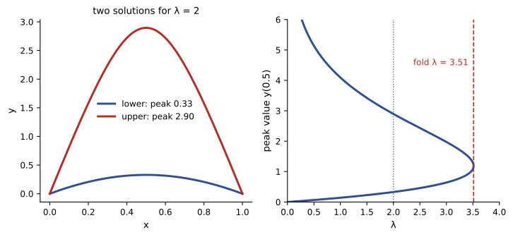
Answer: The two starts converge to two different solutions, a low-temperature one (peak 0.33) and a high-temperature one (peak 2.90). The problem has two solutions for λ below a critical value of about 3.51, and none above it: beyond that, the slab cannot reach a steady state and ignites. Numerical results near such a fold must be interpreted with care, and continuation methods, which step λ gradually and use each solution as the next guess, trace the whole family.
import numpy as np

# Bratu problem: y double-prime + lam * exp(y) = 0, y(0) = y(1) = 0 (thermal ignition in a slab)
N, lam = 50, 2.0
h = 1.0 / N
x = np.linspace(0, 1, N + 1)[1:-1]

def newton(y):
    for it in range(1, 50):
        F = np.zeros(N - 1)
        F[:] = -2 * y + lam * h**2 * np.exp(y)
        F[1:] += y[:-1]
        F[:-1] += y[1:]
        J = np.diag(-2 + lam * h**2 * np.exp(y)) + np.diag(np.ones(N - 2), 1) + np.diag(np.ones(N - 2), -1)
        dy = np.linalg.solve(J, -F)
        y = y + dy
        if np.max(np.abs(dy)) < 1e-12:
            return y, it
    return y, it

for name, guess in [("zero guess", np.zeros(N - 1)), ("large guess", 8 * x * (1 - x) * 4)]:
    y, its = newton(guess)
print(f"{name:11s}: converged in {its} Newton steps, peak value y(0.5) = {y.max():.4f}")zero guess : converged in 5 Newton steps, peak value y(0.5) = 0.3290 large guess: converged in 12 Newton steps, peak value y(0.5) = 2.8951
Eigenvalue problems from BVPs
A homogeneous BVP containing a parameter, such as the buckling equation \(EI\,y'' + Py = 0\) with pinned ends, has non-zero solutions only for particular parameter values (MATH-201). Discretizing it gives a matrix eigenvalue problem. With the centred second difference and \(y_0 = y_N = 0\):
so the buckling loads are the eigenvalues of the tridiagonal matrix on the left, and the eigenvectors are the buckled shapes sampled at the grid points. For a uniform column the smallest eigenvalue converges to the Euler load \(\pi^2EI/L^2\) with error proportional to \(h^2\). The real value of the method is for non-uniform problems: a tapered column, a pile in soil, a shaft with varying diameter, where EI varies along the length and no formula exists. Then \(EI_i\) simply varies from row to row, and the shifted inverse iteration of Lesson 4 finds the lowest loads. Vibration modes of strings, bars and beams are found the same way.
Library solvers
In practice, scipy.integrate.solve_bvp solves nonlinear BVPs by collocation: it represents the solution by piecewise cubic polynomials, requires the equation to hold at chosen points in each interval, and adapts the mesh until a tolerance is met. It needs the problem written as a first-order system, the boundary conditions as a residual function, and an initial guess for the solution on a mesh. A good guess, often from a simplified linear problem or physical intuition, matters as much here as for Newton's method, and the warnings about multiple solutions apply equally.
Common mistakes
MistakeAssuming a BVP always has exactly one solution.
InsteadNonlinear BVPs may have several solutions or none; check with different guesses.
MistakeUsing a one-sided difference for a derivative boundary condition.
InsteadUse a ghost point and a centred difference to keep second-order accuracy.
MistakeSolving a tridiagonal system with a dense solver for large N.
InsteadUse a banded or sparse solver, which costs O(N).
MistakeShooting over a long interval with rapidly growing solutions.
InsteadUse multiple shooting or finite differences instead.
MistakeTrusting a solution without a grid refinement check.
InsteadHalve h and confirm the error falls by about 4 for second-order methods.
Summary and key terms
- Shooting turns a BVP into root finding for the missing initial condition, using an IVP solver.
- A projectile aimed at a target can have two solutions or none.
- Finite differences replace derivatives with differences, giving a tridiagonal system with O(h²) error.
- Fixed-value conditions are substituted directly; derivative conditions use ghost points.
- Nonlinear finite difference systems are solved by Newton's method; different guesses may give different solutions.
- Discretizing a parameter-dependent BVP gives a matrix eigenvalue problem for buckling loads or frequencies.
- solve_bvp uses collocation with mesh adaptation and needs a good initial guess.
- Boundary value problem
- A differential equation with conditions given at more than one point.
- Shooting method
- Solving a BVP by adjusting initial conditions of an IVP until the far condition is met.
- Multiple shooting
- Shooting on subintervals joined by matching conditions.
- Dirichlet condition
- A boundary condition fixing the value of the solution.
- Neumann condition
- A boundary condition fixing the derivative of the solution.
- Ghost point
- A fictitious grid point outside the domain used to impose a derivative condition.
- Tridiagonal system
- A linear system whose matrix is non-zero only on three central diagonals.
- Continuation method
- Tracing a family of solutions by gradually changing a parameter.
- Collocation
- Requiring an approximate solution to satisfy the equation at selected points.
Practice problems
Work each problem on paper first, then reveal the answer to check.
For a linear BVP, how many shots are needed to find the exact initial slope?
Show answer
Two, followed by linear interpolation.
Shots with slopes 1 and 3 give y(b) = 4 and 10; the target is 7. What slope is needed (linear problem)?
Show answer
s = 2.
Write the finite difference equation for y″ = 6x at an interior point.
Show answer
(y_{i−1} − 2yᵢ + y_{i+1})/h² = 6xᵢ.
Solve y″ = 2, y(0) = y(1) = 0 with h = 0.5 by finite differences.
Show answer
One unknown: (0 − 2y₁ + 0)/0.25 = 2, y₁ = −0.25 (exact, since the solution is quadratic).
How does the ghost point implement y′(L) = 0?
Show answer
It sets y_{N+1} = y_{N−1} in the equation at x_N.
A finite difference error is 8 × 10⁻⁴ with N = 20. Estimate it with N = 80.
Show answer
8 × 10⁻⁴/16 = 5 × 10⁻⁵.
What does the Jacobian diagonal become for y″ + y³ = 0 discretized centrally?
Show answer
−2/h² + 3yᵢ².
For the Bratu problem with λ = 4, how many steady solutions exist?
Show answer
None; λ exceeds the critical value 3.51.
With N = 4 intervals on a pinned column, what is the size of the buckling eigenvalue matrix?
Show answer
3 × 3 (the interior points).
Name two reasons to prefer finite differences over shooting.
Show answer
Stability for sensitive problems and easy extension to two and three dimensions.
Lesson quiz · 5 questions
Score 60% or more to complete this lesson.
Create a free account to save your progress, take quizzes and earn a certificate.