
STAT-235 · Lesson 3 of 5 · 37 min
Random variables and distributions
Lesson 1 described data that had already been collected; Lesson 2 gave the rules of probability. This chapter joins them. A random variable attaches a number to each outcome of an uncertain process: the number of defective parts in a sample, the number of vehicles arriving at a ramp in a minute, the life of a bearing, the strength of a concrete cylinder. A probability distribution says how likely each value is. A handful of standard distributions model a remarkable range of engineering situations, and knowing which one fits, and why, is a core engineering skill.
Discrete random variables
A discrete random variable takes countable values (0, 1, 2, …). Its probability mass function (pmf) \(p(x) = P(X = x)\) lists the probability of each value; the probabilities sum to 1. The two most important summaries are the mean (expected value) and the variance:
The mean is the long-run average value; the standard deviation \(\sigma\) measures spread, exactly as for data in Lesson 1, but now for the whole population of possible outcomes rather than one sample.
Worked problem
Trucks at a weigh scale
The number of trucks arriving at a weigh station in a 5-minute interval has pmf: P(0) = 0.10, P(1) = 0.30, P(2) = 0.35, P(3) = 0.15, P(4) = 0.10. Find the mean, the standard deviation, and the probability of 3 or more trucks.
Show solution
- \(\mu = 0(0.10) + 1(0.30) + 2(0.35) + 3(0.15) + 4(0.10) = 1.85\).
- \(\sigma^2 = (1.85)^2(0.10) + (0.85)^2(0.30) + (0.15)^2(0.35) + (1.15)^2(0.15) + (2.15)^2(0.10) = 1.2275\), so \(\sigma = 1.11\).
- P(X ≥ 3) = 0.15 + 0.10 = 0.25.
Answer: Mean 1.85 trucks, standard deviation 1.11 trucks; a quarter of 5-minute intervals have 3 or more trucks, which sets how much queue space the scale needs
The binomial distribution
Many problems count successes in a fixed number of independent trials, each with the same probability: defective items in a sample, days with rain in a week, components that survive a test. If there are n trials with success probability p, the number of successes X is binomial:
The binomial coefficient counts the arrangements of k successes among n trials (Lesson 2), and \(p^k(1 - p)^{n - k}\) is the probability of any one arrangement.
Worked problem
Sampling fasteners
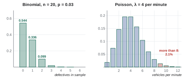
A supplier's bolts are 3% defective. An inspector checks a random sample of 20. Find the probability of no defectives, of exactly one, and of two or more.
Show solution
- P(0) = \(0.97^{20} = 0.544\).
- P(1) = \(20(0.03)(0.97)^{19} = 0.336\).
- P(X ≥ 2) = 1 − 0.544 − 0.336 = 0.120.
- Mean \(np = 0.6\), standard deviation \(\sqrt{20(0.03)(0.97)} = 0.76\).
Answer: P(0) = 0.544, P(1) = 0.336, P(≥2) = 0.120. More than half the samples contain no defective at all, even though 3% of the bolts are bad: a sample of 20 is weak evidence of good quality
The Poisson distribution
When events occur randomly and independently in time or space at an average rate λ (per minute, per kilometre, per square metre), the number of events in an interval follows the Poisson distribution:
Vehicle arrivals at light traffic, calls to a service desk, flaws along a pipeline weld, cracks per square metre of pavement, and large earthquakes in a region are all modelled this way. The Poisson distribution is also the limit of the binomial when n is large and p small, with λ = np: for 1000 items at 0.2% defective, both give P(0) = 0.135.
Worked problem
Sizing a ramp queue
Vehicles arrive at a metered on-ramp at an average of 4 per minute, independently. Find the probability that no vehicles arrive in a minute, that more than 6 arrive, and the storage (in vehicles) that covers at least 95% of minutes.
Show solution
- P(0) = \(e^{-4} = 0.018\).
- P(X > 6) = 1 − P(X ≤ 6) = 1 − 0.889 = 0.111.
- P(X ≤ 7) = 0.949 and P(X ≤ 8) = 0.979, so 8 vehicles is the smallest storage that covers 95%.
Answer: P(0) = 1.8%, P(>6) = 11%; storage for 8 vehicles covers about 98% of minutes. Traffic engineers size turn bays and ramp storage with exactly this reasoning
Continuous random variables
A continuous random variable, such as a strength, a time or a length, can take any value in a range. Probability is now an area under a probability density function (pdf) f(x):
The probability of any single exact value is zero; only intervals have probability. The cumulative distribution function \(F(x) = P(X \le x)\) accumulates the area from the left. The mean and variance use integrals in place of sums: \(\mu = \int x f(x)\,dx\) and \(\sigma^2 = \int (x - \mu)^2 f(x)\,dx\).
The exponential distribution and component life
The time between Poisson events, or the life of a component that fails at a constant rate λ (no wear-out, no infant mortality), is exponential:
R(t) is the reliability function. The mean life 1/λ is called the mean time to failure (MTTF). The exponential distribution is memoryless: a component that has survived 1000 hours is as good as new, which is a reasonable model for electronics during their useful life but not for parts that wear, such as bearings and brake pads. Those are usually modelled with the Weibull distribution, which allows a failure rate that rises or falls with age.
Worked problem
Sensor life
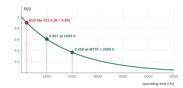
A pressure sensor has a constant failure rate with MTTF 2000 hours. Find the probability that it survives 1000 hours, the probability it survives to the mean life, and the B10 life (the time by which 10% have failed).
Show solution
- λ = 1/2000 per hour. \(R(1000) = e^{-0.5} = 0.607\).
- \(R(2000) = e^{-1} = 0.368\).
- B10: \(e^{-t/2000} = 0.90\), so \(t = -2000 \ln 0.90 = 211\) h.
Answer: R(1000 h) = 0.61, R(2000 h) = 0.37, B10 life 211 h. The mean life is not a "typical" life: 63% of sensors fail before it. Replacement schedules use B-lives instead
The normal distribution
The normal (Gaussian) distribution is the familiar symmetric bell curve with mean μ and standard deviation σ:
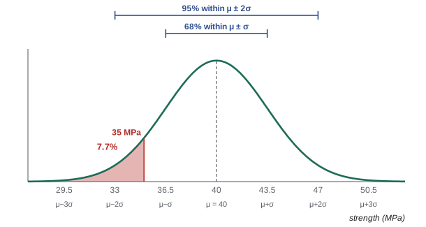
It describes measurement errors, manufacturing dimensions, and many material properties, and, through the central limit theorem below, averages of almost anything. About 68% of values lie within one σ of the mean, 95% within two (more precisely 1.96σ) and 99.7% within three.
Every normal distribution becomes the standard normal (mean 0, standard deviation 1) by the z-transformation of Lesson 1:
Φ(z) is the standard normal CDF, tabulated in every statistics text and available as NORM.S.DIST in spreadsheets and scipy.stats.norm.cdf in Python. Useful values: Φ(1.645) = 0.95, Φ(1.96) = 0.975, Φ(2.326) = 0.99.
Worked problem
Concrete below specified strength
A ready-mix plant's 28-day cylinder strengths are normal with mean 40 MPa and standard deviation 3.5 MPa. What fraction of cylinders fall below 35 MPa? What strength is exceeded by 90% of cylinders?
Show solution
- \(z = (35 - 40)/3.5 = -1.43\), so \(P(X < 35) = \Phi(-1.43) = 0.077\).
- The 10th percentile has \(z = -1.2816\): \(x = 40 - 1.2816(3.5) = 35.5\) MPa.
Answer: 7.7% of cylinders test below 35 MPa; 90% exceed 35.5 MPa
This is why concrete is batched to a mean strength well above the specified strength f′c. ACI 318, for example, requires a target average strength of at least \(f'_c + 1.34s\) (and \(f'_c + 2.33s - 3.5\) MPa), where s is the plant's documented standard deviation. For f′c = 30 MPa and s = 3.5 MPa both rules give about 34.7 MPa. A plant with tighter control (smaller s) can batch closer to f′c and save cement: statistics has a direct price.
Combining random variables
Engineering quantities are often sums or differences of random parts: the length of a stack of parts, the clearance between a shaft and a hole, a total load. For independent variables:
Variances add, even for a difference. Standard deviations therefore combine by root-sum-square: three parts each with σ = 0.05 mm stack to σ = \(\sqrt{3}(0.05) = 0.087\) mm, not 0.15 mm. This is the statistical tolerancing that ENGG-160 contrasted with worst-case stack-up. Sums and differences of independent normal variables are themselves normal.
Worked problem
Shaft and hole clearance
Holes are bored with diameter normal, mean 25.010 mm, σ = 0.004 mm; shafts are turned with mean 24.990 mm, σ = 0.003 mm. Parts are assembled at random. What fraction of assemblies have a clearance less than 0.010 mm?
Show solution
- Clearance C = hole − shaft. Mean 25.010 − 24.990 = 0.020 mm.
- \(\sigma_C = \sqrt{0.004^2 + 0.003^2} = 0.005\) mm.
- \(z = (0.010 - 0.020)/0.005 = -2\), so \(P(C < 0.010) = \Phi(-2) = 0.023\).
Answer: About 2.3% of assemblies are too tight
The central limit theorem
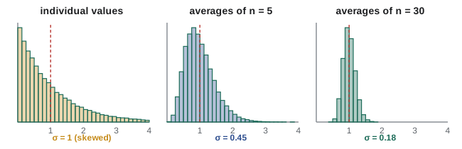
If you average n independent measurements from any distribution with mean μ and standard deviation σ, the average \(\bar{X}\) has mean μ and standard deviation
and, as n grows, its distribution approaches the normal, whatever the shape of the original distribution. This is the central limit theorem, and it is why the normal distribution is everywhere: many measured quantities are effectively sums of many small independent effects, and statistical methods built on averages work even for skewed data once samples are moderately large (n of about 30 is a common rule of thumb; less for symmetric data).
Worked problem
Averages are less variable
Using the plant from the earlier example (μ = 40 MPa, σ = 3.5 MPa), what is the probability that the average of 25 cylinders is below 38.5 MPa?
Show solution
- \(\sigma_{\bar{X}} = 3.5/\sqrt{25} = 0.70\) MPa.
- \(z = (38.5 - 40)/0.70 = -2.14\), so \(P = \Phi(-2.14) = 0.016\).
Answer: Only 1.6%, though about a third of individual cylinders fall below 38.5 MPa. A low average of 25 tests would be strong evidence that the mix has drifted, the idea behind Lesson 4
Computing distributions in Python
Tables are fine for exams, but in practice probabilities come from software. scipy.stats provides every common distribution with the same interface: pmf or pdf, cdf, ppf (the inverse CDF, for percentiles) and sf (the survival function, 1 − cdf).
from scipy import stats

bolts = stats.binom(n=20, p=0.03)
print(f"Binomial P(0) = {bolts.pmf(0):.3f}, P(>=2) = {bolts.sf(1):.3f}")

ramp = stats.poisson(mu=4)
print(f"Poisson P(>6) = {ramp.sf(6):.3f}, 95th percentile = {ramp.ppf(0.95):.0f}")

concrete = stats.norm(loc=40, scale=3.5)
print(f"Normal P(<35) = {concrete.cdf(35):.3f}, 10th percentile = {concrete.ppf(0.10):.1f} MPa")

sensor = stats.expon(scale=2000)
print(f"Exponential R(1000) = {sensor.sf(1000):.3f}")
Output: Binomial P(0) = 0.544, P(>=2) = 0.120; Poisson P(>6) = 0.111, 95th percentile = 8; Normal P(<35) = 0.077, 10th percentile = 35.5 MPa; Exponential R(1000) = 0.607.
Common mistakes
MistakeUsing the binomial when trials are not independent or p changes.
InsteadCheck the conditions: fixed n, independent trials, constant p. Sampling without replacement from a small lot needs the counting method of Lesson 2.
MistakeTreating a pdf value as a probability.
InsteadFor continuous variables, probability is area under the pdf; f(x) itself can exceed 1.
MistakeAdding standard deviations of independent parts.
InsteadAdd variances; standard deviations combine by root-sum-square.
MistakeAssuming the mean life is a typical life for exponential failures.
InsteadOnly 37% survive to the MTTF; use percentile (B) lives for maintenance planning.
MistakeAssuming normality for skewed quantities, especially in the tails.
InsteadCheck the data; floods, winds and fatigue lives usually need skewed models.
MistakeForgetting √n when working with averages.
InsteadThe standard deviation of a mean of n values is σ/√n.
Summary and key terms
- A random variable assigns numbers to uncertain outcomes; its distribution gives probabilities, with mean μ and variance σ².
- Binomial: successes in n independent trials with probability p; mean np, variance np(1 − p).
- Poisson: random events at average rate λ; mean and variance both λ. Approximates the binomial for large n and small p.
- For continuous variables, probability is area under the pdf. Exponential life: R(t) = e^(−λt), memoryless, MTTF = 1/λ.
- Normal: standardize with z = (x − μ)/σ and use Φ(z); 68–95–99.7% within 1, 2, 3 σ.
- Independent variances add for sums and differences; averages of n values have standard deviation σ/√n and are approximately normal by the central limit theorem.
- Random variable
- A numerical value determined by the outcome of an uncertain process.
- Probability mass function
- P(X = x) for each value of a discrete random variable.
- Probability density function
- A curve whose area over an interval gives the probability of that interval.
- Cumulative distribution function
- F(x) = P(X ≤ x).
- Expected value
- The long-run mean of a random variable.
- Binomial distribution
- The number of successes in n independent trials with constant probability p.
- Poisson distribution
- The number of random independent events in an interval at average rate λ.
- Exponential distribution
- The time to failure at a constant failure rate.
- Reliability function
- R(t) = P(T > t), the probability of surviving beyond time t.
- Normal distribution
- The symmetric bell-shaped distribution with mean μ and standard deviation σ.
- Standard normal
- The normal distribution with mean 0 and standard deviation 1.
- Central limit theorem
- Averages of many independent values are approximately normal, with standard deviation σ/√n.
Practice problems
Work each problem on paper first, then reveal the answer to check.
X takes values 1, 2, 3 with probabilities 0.2, 0.5, 0.3. Find E[X] and Var(X).
Show answer
E[X] = 2.1; E[X²] = 0.2 + 2.0 + 2.7 = 4.9; Var = 4.9 − 4.41 = 0.49.
A test has 10 multiple-choice questions with 4 options each. Guessing at random, what is the probability of getting exactly 3 right?
Show answer
C(10, 3)(0.25)³(0.75)⁷ = 120 × 0.015625 × 0.1335 = 0.250.
Of the welds made by a robot, 1% need repair. In a batch of 50, find the mean and standard deviation of the number needing repair.
Show answer
Mean 0.5; σ = √(50 × 0.01 × 0.99) = 0.70.
Flaws occur along a pipeline weld at 0.5 per 100 m. What is the probability that a 300 m section has no flaws?
Show answer
λ = 1.5; P(0) = e^(−1.5) = 0.223.
A call centre receives 6 calls per hour on average. What is the probability of exactly 6 calls in an hour?
Show answer
e^(−6)6⁶/6! = 0.161.
A fan motor has a constant failure rate of 0.0001 per hour. Find its MTTF and its reliability for 5000 hours.
Show answer
MTTF = 10 000 h; R = e^(−0.5) = 0.607.
Resistor values are normal with mean 100 Ω and standard deviation 2 Ω. What fraction lies between 97 and 103 Ω?
Show answer
z = ±1.5; Φ(1.5) − Φ(−1.5) = 0.866.
For the resistors in the previous problem, what value is exceeded by only 1%?
Show answer
100 + 2.326 × 2 = 104.7 Ω.
Four blocks, each with length standard deviation 0.02 mm, are stacked. Find the standard deviation of the stack height.
Show answer
√4 × 0.02 = 0.04 mm.
Individual measurements have σ = 6 units. How many must be averaged for the standard deviation of the average to be 1.5 units?
Show answer
σ/√n = 1.5 → √n = 4 → n = 16.
Lesson quiz · 5 questions
Score 60% or more to complete this lesson.
Create a free account to save your progress, take quizzes and earn a certificate.