
ENGG-401 · Lesson 9 of 12 · 24 min
Depreciation and income taxes
Taxes are often one of the largest cash flows of a business investment, and they can change which alternative is best. Income taxes are levied on profits, and the tax system allows businesses to deduct the cost of capital assets gradually over time through depreciation, called capital cost allowance in Canada. Because the timing of these deductions affects the present worth of tax savings, tax rules have a direct effect on engineering decisions about equipment, buildings and technology. This lesson explains depreciation as an accounting and tax concept, the main depreciation methods, the tax depreciation systems of Canada and the United States, corporate income tax rates, after-tax cash flows, the tax shield, disposals, recapture and losses, and how to perform after-tax analysis with an after-tax MARR. Tax rules change frequently; the figures here are current as of late 2026 and must always be confirmed for a real analysis.
What depreciation is
Depreciation is the allocation of the cost of a capital asset over its useful life. It is not a cash flow: the cash is spent when the asset is bought. But depreciation matters in two ways. For financial reporting, it spreads the cost of assets over the years they help earn revenue, giving a truer picture of profit. For taxes, depreciation deductions reduce taxable income and therefore taxes, which are real cash flows. Tax depreciation rules are set by legislation and often differ from accounting depreciation; engineering economic analyses use tax depreciation to calculate after-tax cash flows.
Classical depreciation methods
Three classical methods illustrate how depreciation can be spread:
- Straight-line (SL): equal deductions each year, \(D_t = (P - S)/n\), where \(P\) is first cost, \(S\) estimated salvage and \(n\) the life. Simple and common in financial reporting.
- Declining balance (DB): a constant percentage \(d\) of the remaining book value each year, \(D_t = d \times BV_{t-1}\). Double declining balance uses \(d = 2/n\). Deductions are larger early and smaller later, matching assets that lose value quickly.
- Sum-of-years-digits (SOYD): deductions proportional to the remaining years of life; rarely used for tax today but common in textbooks.
Accelerated methods, which give larger deductions early, are worth more to a taxpaying firm because tax savings arrive sooner. This is why governments use accelerated depreciation and immediate expensing as investment incentives.
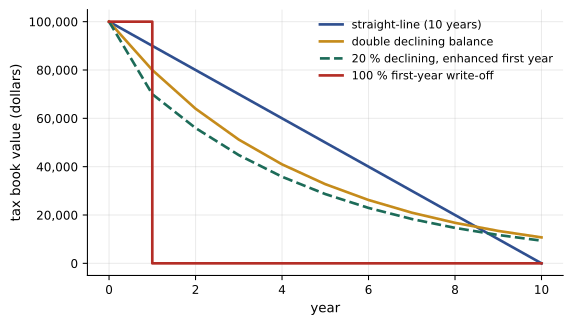
Tax depreciation systems
In the United States, tax depreciation follows the Modified Accelerated Cost Recovery System (MACRS) under the Internal Revenue Code. Assets are assigned recovery periods, such as 3, 5, 7, 10, 15 and 20 years for personal property, 27.5 years for residential rental property and 39 years for non-residential real property. Personal property generally uses the 200 % declining balance method switching to straight-line, with a half-year convention that treats assets as placed in service at mid-year, and IRS tables give the annual percentages. On top of MACRS, bonus depreciation and Section 179 expensing allow immediate deductions: the One Big Beautiful Bill Act (signed 4 July 2025) made 100 % bonus depreciation permanent for qualifying property acquired after 19 January 2025, and the Section 179 limit for 2026 is $2,560,000, phasing out dollar for dollar above $4,090,000 of qualifying purchases (Rev. Proc. 2025-32).
| Year | 7-year MACRS rate | Deduction on $100,000 | With 100 % bonus |
|---|---|---|---|
| 1 | 14.29 % | 14,290 | 100,000 |
| 2 | 24.49 % | 24,490 | 0 |
| 3 | 17.49 % | 17,490 | 0 |
| 4 | 12.49 % | 12,490 | 0 |
| 5 | 8.93 % | 8,930 | 0 |
| 6 | 8.92 % | 8,920 | 0 |
| 7 | 8.93 % | 8,930 | 0 |
| 8 | 4.46 % | 4,460 | 0 |
Corporate income tax rates
The tax rate used in analysis is the marginal rate on the firm's additional income, combining all levels of government.
In the United States, the federal corporate income tax rate is a flat 21 %, and most states levy their own corporate income taxes, typically between about 2 % and 11 %; because state taxes are deductible for federal purposes, the combined marginal rate is \(t = t_f + t_s (1 - t_f)\), roughly 25 % to 28 % for many firms. Pass-through businesses such as partnerships, S corporations and sole proprietorships are taxed at owners' individual rates instead.
After-tax cash flows
The after-tax cash flow (ATCF) in each year is the before-tax cash flow minus income taxes, where taxes are calculated on taxable income, which is before-tax cash flow minus tax depreciation:
The second form is especially useful: the after-tax cash flow equals the before-tax cash flow reduced by the tax rate, plus the tax saving from depreciation, \(t D_t\), called the depreciation tax shield. First costs are not deducted directly (except under immediate expensing); their effect appears through the depreciation tax shield over time.
The present worth of the tax shield
Because depreciation deductions occur over many years, their present worth depends on the method and the discount rate. Faster deductions are worth more.
For MACRS, the present worth of the tax shield is the sum of \(t\,P\,r_k/(1 + i)^k\) over the recovery years, where \(r_k\) are the table rates. For a $100,000 7-year asset at \(t = 25\,\%\) and \(i = 10\,\%\), the MACRS shield is worth about $18,040, while 100 % bonus depreciation gives a deduction of $100,000 in year 1 with a shield worth about $22,730, the maximum possible because the entire cost is deducted at once.
Disposals: recapture, gains and losses
When an asset is sold, the sale price is compared with its tax book value.
In the United States, the gain on sale is the sale price minus the adjusted basis (cost minus accumulated depreciation). For personal property (Section 1245), the part of the gain up to accumulated depreciation is recaptured as ordinary income; any excess above original cost is a capital gain. A sale below adjusted basis gives a deductible loss. With 100 % bonus depreciation, the adjusted basis is zero, so the entire sale price of a used asset is typically taxable as ordinary income.
Performing an after-tax analysis
Worked problem
After-tax evaluation of the inspection system
Reconsider the $80,000 inspection system with $22,000 annual savings and a $10,000 salvage value after 6 years. The firm elects 100 % bonus depreciation, the combined tax rate is 25 %, and the after-tax MARR is 7.5 %. Find the after-tax cash flows, present worth and rate of return.
Show solution
- Year 1 depreciation: the full $80,000, giving a tax saving of \(0.25 \times 80{,}000 = 20{,}000\).
- Annual after-tax savings: \(22{,}000 \times 0.75 = 16{,}500\); year 1 ATCF = \(16{,}500 + 20{,}000 = 36{,}500\).
- Year 6 salvage of $10,000 is fully recaptured as ordinary income: after tax \(10{,}000 \times 0.75 = 7{,}500\), so year 6 ATCF = 24,000.
- PW at 7.5 % ≈ +$20,900 and after-tax IRR ≈ 16.6 %, above the after-tax MARR.
Answer: The investment remains attractive after tax, with an after-tax IRR of about 16.6 %.
After-tax MARR and practical points
After-tax cash flows must be discounted at an after-tax MARR, which is lower than the before-tax MARR. A rough approximation is \(\text{MARR}_{\text{after}} \approx \text{MARR}_{\text{before}} \times (1 - t)\), though firms usually set the after-tax MARR directly from their after-tax cost of capital. Other practical points include: interest on debt is tax-deductible, but in most project analyses financing is excluded and reflected in the MARR instead, to avoid double counting; tax losses on a project can usually offset other income of a profitable firm, so negative taxable income generates tax savings; investment tax credits, such as clean technology credits in both countries, reduce taxes directly and usually also reduce the depreciable cost; and leasing changes the tax picture because lease payments are deductible while the lessor claims depreciation. Because tax rules are complex and change frequently, real analyses should be reviewed by tax specialists.
Leasing versus buying after tax
Taxes are central to lease-versus-buy decisions. When a firm buys equipment, it pays the purchase price and claims tax depreciation; when it leases under an operating lease, it pays lease payments that are usually deductible as an expense, and the lessor claims the depreciation. An after-tax comparison discounts each option's after-tax cash flows, typically at the after-tax cost of borrowing, because a lease is a substitute for debt financing. Leasing can be attractive when the lessee cannot use tax deductions efficiently, for example because it has losses, or when the lessor can obtain equipment more cheaply, offers maintenance, or bears the risk of obsolescence. Accounting standards now require most leases to appear on the balance sheet, but the tax and cash flow analysis remains the basis of the economic decision.
Investment tax credits and incentives
Governments use tax credits and incentives to encourage particular investments, such as clean energy, research and development, manufacturing and regional development. An investment tax credit reduces taxes payable directly by a percentage of eligible spending, and usually also reduces the cost base for tax depreciation. Other incentives include accelerated or immediate expensing, grants that reduce the net first cost, and production-based credits paid per unit of output. Engineers should identify which incentives apply to their projects and include them as cash flows, while recognizing that incentive programs often have detailed eligibility conditions, application processes, recapture provisions if conditions are not met, and expiry dates that change with government budgets. A project that is attractive only because of an incentive scheduled to expire carries policy risk that should be included in sensitivity analysis.
A systematic after-tax table
A clear way to organize after-tax analysis is a table with one row per year and columns for before-tax cash flow, tax depreciation, taxable income, income tax and after-tax cash flow. The first cost appears in year 0, depreciation in each year according to the tax rules, the disposal proceeds and any recapture or loss in the final year, and the after-tax cash flows are then discounted at the after-tax MARR. Laying out each step makes errors visible and lets reviewers check the calculation.
Taxes and the choice of alternatives
Taxes can change the ranking of alternatives, not just their values. Because operating costs are deductible immediately while capital costs are deducted gradually, a capital-intensive alternative loses some of its advantage after tax under slow depreciation and gains under immediate expensing. Similarly, an alternative eligible for an investment tax credit may become preferred after tax. For this reason, important decisions should be analyzed after tax with the rules that will actually apply, rather than assuming that before-tax rankings will hold.
Depreciation and financial statements
Firms typically keep two sets of depreciation records: tax depreciation for tax returns and accounting depreciation for financial statements, often straight-line over useful lives. Differences between them create deferred tax balances on the balance sheet. For engineering economic analysis, only tax depreciation affects cash flows, so engineers should obtain the tax treatment of an asset from their finance or tax department rather than using the accounting schedule, and should recognize that managers may also care about the effect of a project on reported earnings, which depends on accounting depreciation.
Because tax law changes frequently, many firms maintain an internal guide to the depreciation treatment of common asset types, updated each year by their tax advisers. Engineers preparing economic studies should consult it, record which version of the rules they applied and note any incentives whose expiry or phase-out could affect the result, so that the analysis can be updated if legislation changes before the investment is made.
Common mistakes
MistakeTreating depreciation as a cash outflow.
InsteadDepreciation affects cash only through taxes.
MistakeUsing straight-line depreciation for tax calculations.
InsteadUse the jurisdiction's tax depreciation rules.
MistakeDiscounting after-tax cash flows at a before-tax MARR.
InsteadUse an after-tax MARR.
MistakeIgnoring tax on salvage or recapture.
InsteadApply disposal rules to the sale proceeds.
MistakeRelying on old tax rates and incentives.
InsteadConfirm current legislation for every analysis.
Summary and key terms
- Depreciation allocates asset cost over time and affects cash through taxes.
- Straight-line, declining balance and SOYD spread deductions differently.
- Canada uses pooled CCA classes; the US uses MACRS with bonus and Section 179.
- Accelerated and immediate deductions are worth more in present worth terms.
- ATCF = BTCF (1 − t) + t D, where t D is the depreciation tax shield.
- Disposals trigger recapture, gains or losses under each country's rules.
- Discount after-tax cash flows at an after-tax MARR and verify current rules.
- Depreciation
- Allocation of an asset's cost over its life.
- Book value
- Cost minus accumulated depreciation.
- Straight-line
- Equal depreciation each year.
- Declining balance
- Constant percentage of remaining book value.
- Capital cost allowance
- Canadian tax depreciation.
- MACRS
- US Modified Accelerated Cost Recovery System.
- Bonus depreciation
- Immediate deduction of a percentage of cost.
- Tax shield
- Tax saving from a deduction, t × D.
- Recapture
- Previously deducted depreciation taxed on disposal.
- After-tax MARR
- Minimum return required on after-tax cash flows.
Practice problems
Work each problem on paper first, then reveal the answer to check.
Straight-line depreciation of $60,000 with $10,000 salvage over 5 years?
Show answer
$10,000 per year.
Double declining balance rate for a 10-year life?
Show answer
20 %.
Why are accelerated deductions valuable?
Show answer
Tax savings arrive sooner and have higher present worth.
Write the ATCF formula.
Show answer
ATCF = BTCF (1 − t) + t D.
Tax shield of a $40,000 deduction at 25 %?
Show answer
$10,000.
First-year MACRS deduction on $50,000 of 5-year property without bonus?
Show answer
20 % × 50,000 = $10,000.
How is gain up to accumulated depreciation taxed for Section 1245 property?
Show answer
As ordinary income (recapture).
Approximate after-tax MARR for 12 % before tax at 25 % tax?
Show answer
About 9 %.
Why exclude financing from most project cash flows?
Show answer
It is reflected in the MARR; including it double counts.
Why must tax rules be checked for every analysis?
Show answer
They change frequently.
Lesson quiz · 5 questions
Score 60% or more to complete this lesson.
Create a free account to save your progress, take quizzes and earn a certificate.