Orthogonality and least squares

Measured data never fit a model exactly. A spring tested at ten loads gives ten points that lie close to, but not on, a straight line; a survey network with redundant measurements gives slightly conflicting coordinates; a set of temperature readings scatters around a trend. The corresponding linear systems have more equations than unknowns and no exact solution. The method of least squares, developed independently by Legendre and Gauss around 1800 to fit planetary orbits and survey the Earth, finds the solution that comes closest, in the sense of minimizing the sum of squared errors. Its theory rests on orthogonality: the best approximation is the one whose error is perpendicular to everything the model can produce. This lesson develops orthogonal vectors and projections, the Gram-Schmidt process and QR factorization, and the normal equations of least squares, and applies them to fitting lines, curves and survey networks.

Orthogonal vectors and subspaces

Two vectors are orthogonal if their dot product is zero (Lesson 1). A set of vectors is orthogonal if every pair is orthogonal, and orthonormal if, in addition, every vector has length 1. Orthogonal sets of non-zero vectors are automatically linearly independent, and coordinates with respect to an orthonormal basis are simply dot products (Lesson 2), which makes such bases exceptionally convenient.

A vector is orthogonal to a subspace if it is orthogonal to every vector in it, which is equivalent to being orthogonal to each vector in a basis of the subspace. The set of all such vectors is the orthogonal complement. For example, in \(\mathbb{R}^3\), the orthogonal complement of a plane through the origin is the line along its normal vector. A key fact connects this to the subspaces of Lesson 7: the null space of a matrix is the orthogonal complement of its row space, since \(A\mathbf{x} = \mathbf{0}\) says exactly that \(\mathbf{x}\) is orthogonal to every row of \(A\).

Projection onto a subspace

Lesson 8 projected a vector onto a line. More generally, the orthogonal projection of a vector \(\mathbf{b}\) onto a subspace \(W\) is the vector \(\hat{\mathbf{b}}\) in \(W\) closest to \(\mathbf{b}\). It is characterized by a simple geometric condition: the error \(\mathbf{b} - \hat{\mathbf{b}}\) is orthogonal to \(W\). The distance from \(\mathbf{b}\) to the subspace is the length of this error, by the Pythagorean theorem, since the error is perpendicular to every other displacement within \(W\).

If \(W\) has an orthogonal basis \(\mathbf{u}_1, \ldots, \mathbf{u}_k\), the projection is the sum of the projections onto each basis vector:

The Gram-Schmidt process and QR factorization

The projection formula needs an orthogonal basis. The Gram-Schmidt process builds one from any basis: take the first vector as it is; from the second, subtract its projection onto the first; from the third, subtract its projections onto the first two new vectors; and so on. Each step removes the components along earlier directions, leaving a vector orthogonal to them. Dividing each result by its length gives an orthonormal basis.

Recording the Gram-Schmidt process in matrix form gives the QR factorization \(A = QR\), where \(Q\) has orthonormal columns and \(R\) is upper triangular. It plays the role for least squares that LU plays for square systems (Lesson 5), and numerical libraries compute it with more stable variants, such as Householder reflections, rather than classical Gram-Schmidt, which can lose orthogonality to rounding errors.

The least squares problem

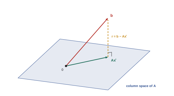
Suppose \(A\mathbf{x} = \mathbf{b}\) has more equations than unknowns and no exact solution: \(\mathbf{b}\) is not in the column space of \(A\) (Lesson 7). The least squares solution is the vector \(\hat{\mathbf{x}}\) that makes \(A\hat{\mathbf{x}}\) as close as possible to \(\mathbf{b}\), minimizing the length of the residual \(\mathbf{r} = \mathbf{b} - A\mathbf{x}\), equivalently the sum of the squared residuals \(\sum r_i^2\).

Geometrically, \(A\hat{\mathbf{x}}\) is the projection of \(\mathbf{b}\) onto the column space, so the residual must be orthogonal to every column of \(A\): \(A^T(\mathbf{b} - A\hat{\mathbf{x}}) = \mathbf{0}\). Rearranging gives the normal equations:

If the columns of \(A\) are independent, \(A^TA\) is a square, symmetric, invertible (indeed positive definite) matrix, and the normal equations have a unique solution. For small problems they are solved directly; for large or ill-conditioned problems, the QR factorization is preferred, because forming \(A^TA\) squares the condition number (Lesson 5): with \(A = QR\), the least squares solution satisfies \(R\hat{\mathbf{x}} = Q^T\mathbf{b}\).

Fitting a straight line

To fit a line \(y = c_0 + c_1 t\) to data points \((t_i, y_i)\), each point gives one equation \(c_0 + c_1 t_i = y_i\). With \(m\) points this is the system \(A\mathbf{c} = \mathbf{y}\), where \(A\) has a column of ones and a column of the \(t_i\). The normal equations become:

The quality of a fit is judged from its residuals. A pattern in the residuals, such as all positive at the ends and negative in the middle, means the model is missing something, perhaps curvature. The root-mean-square residual estimates the measurement noise, and the coefficient of determination \(R^2\) measures the fraction of the variation explained by the model. STAT-235 develops the statistics of fitted models, including confidence intervals for the coefficients.

Fitting curves and models

Least squares applies to any model that is linear in its unknown coefficients, even if it is not linear in the variable. A quadratic \(y = c_0 + c_1t + c_2t^2\) gives a matrix with columns \(1\), \(t_i\) and \(t_i^2\). A periodic model \(y = c_0 + c_1\cos\omega t + c_2\sin\omega t\), used to fit daily temperature cycles or tidal records, gives columns \(1\), \(\cos\omega t_i\), \(\sin\omega t_i\). Models that are not linear in their coefficients can sometimes be transformed: the exponential \(y = Ae^{kt}\) becomes linear after taking logarithms, \(\ln y = \ln A + kt\) (MATH-100, Lesson 2), though the transformation changes how errors are weighted.

Adding more terms always reduces the residuals on the data used for fitting, but beyond a point it fits the noise rather than the underlying behavior, a problem called overfitting. A polynomial of degree \(m - 1\) passes exactly through \(m\) points but usually oscillates wildly between them. The cure is to choose models with physical justification, use as few parameters as the data require, and check predictions against data not used in the fit, ideas that are central to machine learning (AI-210).

Weighted least squares

Ordinary least squares treats every measurement as equally reliable. When some measurements are more precise than others, for example a distance measured by laser alongside one measured by tape, it is better to give each squared residual a weight inversely proportional to the variance of that measurement. Minimizing \(\sum w_i r_i^2\) leads to the weighted normal equations \(A^TWA\,\hat{\mathbf{x}} = A^TW\mathbf{b}\), where \(W\) is the diagonal matrix of weights. Survey adjustments, GPS positioning and sensor fusion all use weighted least squares, and the Kalman filter used in navigation is a recursive form of it that updates the estimate as each new measurement arrives. The same theory also gives the uncertainty of the fitted values: the matrix \((A^TWA)^{-1}\) is their covariance matrix, which Lesson 11 shows how to interpret through its principal axes.