
MATH-125 · Lesson 11 of 12 · 30 min
Symmetric matrices, principal axes and the SVD
Symmetric matrices, those equal to their own transpose, appear everywhere in engineering: stiffness and mass matrices, stress and strain tensors, inertia tensors, covariance matrices of measurements, and the matrix \(A^TA\) of least squares (Lesson 10). They have exceptionally well-behaved eigenvalues and eigenvectors, a result known as the spectral theorem, which gives every symmetric matrix a set of perpendicular principal axes. Principal axes explain why a loaded material has directions of maximum and minimum stress, why a structure vibrates in distinct mode shapes, why a spinning body has stable axes of rotation, and why the scatter of measured data has a dominant direction. This lesson develops the spectral theorem and its applications, connects symmetric matrices to quadratic forms and energy, and then introduces the singular value decomposition (SVD), which extends the idea of principal axes to every matrix and underlies data compression, model reduction and the reliable solution of difficult least squares problems.
The spectral theorem
Lesson 9 showed that eigenvalues can be complex and that some matrices cannot be diagonalized. Symmetric matrices have neither problem. For a real symmetric matrix \(S = S^T\):
- All eigenvalues are real.
- Eigenvectors belonging to different eigenvalues are orthogonal.
- There is always a full set of orthonormal eigenvectors, so \(S\) can be diagonalized by an orthogonal matrix.
In matrix form, the spectral theorem states:
where \(\Lambda\) is the diagonal matrix of eigenvalues and the columns of the orthogonal matrix \(Q\) (Lesson 8) are the corresponding unit eigenvectors. Geometrically, \(S\) acts by rotating to the eigenvector axes (\(Q^T\)), stretching along each axis by its eigenvalue (\(\Lambda\)), and rotating back (\(Q\)). The eigenvector directions are the principal axes of \(S\). Equivalently, \(S = \sum \lambda_i \mathbf{q}_i\mathbf{q}_i^T\): a symmetric matrix is a weighted sum of projections onto its principal axes.
Worked problem
Diagonalizing a symmetric matrix
Find the eigenvalues and orthonormal eigenvectors of \(S = \begin{pmatrix} 5 & 2 \\ 2 & 2 \end{pmatrix}\).
Show solution
- Characteristic equation (Lesson 9): \(\lambda^2 - 7\lambda + 6 = 0\), so \(\lambda_1 = 6\), \(\lambda_2 = 1\).
- For \(\lambda = 6\): \((S - 6I)\mathbf{v} = 0\) gives \(-v_1 + 2v_2 = 0\), so \(\mathbf{v}_1 = (2, 1)/\sqrt{5}\).
- For \(\lambda = 1\): \(4v_1 + 2v_2 = 0\), so \(\mathbf{v}_2 = (1, -2)/\sqrt{5}\). Check: \(\mathbf{v}_1\cdot\mathbf{v}_2 = (2 - 2)/5 = 0\).
Answer: Eigenvalues 6 and 1 with perpendicular eigenvectors (2, 1)/√5 and (1, −2)/√5, as the spectral theorem promises.
Principal stresses
The state of stress at a point in a loaded plate is described by a symmetric matrix, the stress tensor, containing normal stresses \(\sigma_x\), \(\sigma_y\) and the shear stress \(\tau_{xy}\):
Its eigenvalues are the principal stresses, the largest and smallest normal stresses on any plane through the point, and its eigenvectors are the principal directions, on whose planes the shear stress is zero. Materials such as concrete and cast iron crack perpendicular to the direction of maximum tensile principal stress, and design codes for metals compare combinations of principal stresses with the material's strength.
Worked problem
Principal stresses in a plate
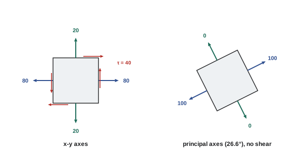
At a point in a steel bracket, \(\sigma_x = 80\) MPa, \(\sigma_y = 20\) MPa and \(\tau_{xy} = 40\) MPa. Find the principal stresses, their directions, and the maximum in-plane shear stress.
Show solution
- Characteristic equation: \(\lambda^2 - 100\lambda + (80 \times 20 - 40^2) = \lambda^2 - 100\lambda + 0 = 0\).
- Principal stresses: \(\sigma_1 = 100\) MPa, \(\sigma_2 = 0\) MPa.
- Direction of \(\sigma_1\): \((80 - 100)v_1 + 40v_2 = 0\) gives \(\mathbf{v} = (2, 1)\), at \(\arctan(1/2) = 26.6°\) from the x-axis.
- Maximum in-plane shear: \((\sigma_1 - \sigma_2)/2 = 50\) MPa, on planes at 45° to the principal directions.
Answer: σ₁ = 100 MPa at 26.6°, σ₂ = 0, and maximum shear 50 MPa. These are the results that Mohr's circle gives graphically in mechanics of materials courses; Mohr's circle is a picture of this eigenvalue problem.
Quadratic forms and definiteness
A symmetric matrix defines a quadratic form \(Q(\mathbf{x}) = \mathbf{x}^T S\mathbf{x}\), a homogeneous quadratic expression in the components of \(\mathbf{x}\); for example, \(5x^2 + 4xy + 2y^2\) corresponds to the matrix in the first example. Quadratic forms represent energies: the strain energy of a structure with stiffness matrix \(K\) and displacements \(\mathbf{u}\) is \(\tfrac{1}{2}\mathbf{u}^TK\mathbf{u}\), and the kinetic energy of a system with mass matrix \(M\) is \(\tfrac{1}{2}\dot{\mathbf{u}}^TM\dot{\mathbf{u}}\).
In the principal axes, the quadratic form has no cross terms: writing \(\mathbf{x} = Q\mathbf{y}\) gives \(Q(\mathbf{x}) = \lambda_1 y_1^2 + \lambda_2 y_2^2 + \cdots\). The signs of the eigenvalues therefore classify the form. If all eigenvalues are positive, the form is positive for every non-zero \(\mathbf{x}\) and \(S\) is positive definite, the property of stiffness matrices of properly supported structures noted in Lesson 5. If some eigenvalues are negative, the form takes both signs; if some are zero, there are directions with no energy, the mechanisms of Lesson 7. The level set \(\mathbf{x}^TS\mathbf{x} = 1\) of a positive definite form is an ellipse (an ellipsoid in three dimensions) whose axes lie along the eigenvectors, with semi-axis lengths \(1/\sqrt{\lambda_i}\).
Vibration modes
A structure with mass matrix \(M\) and stiffness matrix \(K\), both symmetric and positive definite, vibrates freely according to \(M\ddot{\mathbf{u}} + K\mathbf{u} = \mathbf{0}\). Seeking motions in which every point moves in step, \(\mathbf{u} = \boldsymbol{\phi}\cos\omega t\), gives the generalized eigenvalue problem \(K\boldsymbol{\phi} = \omega^2 M\boldsymbol{\phi}\). Its eigenvalues are the squares of the natural frequencies, and its eigenvectors are the mode shapes. Because \(K\) and \(M\) are symmetric, the mode shapes are orthogonal with respect to the mass matrix, so any free vibration is a superposition of independent modes, each oscillating at its own frequency.
Worked problem
Two-story frame
A simple model of a two-story building has equal floor masses \(m\) and story stiffnesses \(k\), giving \(M = mI\) and \(K = k\begin{pmatrix} 2 & -1 \\ -1 & 1 \end{pmatrix}\). Find the natural frequencies and mode shapes.
Show solution
- Eigenvalues of \(\begin{pmatrix} 2 & -1 \\ -1 & 1 \end{pmatrix}\): \(\mu^2 - 3\mu + 1 = 0\), so \(\mu = (3 \mp \sqrt{5})/2 = 0.382\) and \(2.618\).
- Frequencies: \(\omega = \sqrt{\mu k/m}\): \(0.618\sqrt{k/m}\) and \(1.618\sqrt{k/m}\).
- Mode 1 (\(\mu = 0.382\)): \((2 - 0.382)\phi_1 = \phi_2\), so \(\boldsymbol{\phi} = (1, 1.618)\), both floors moving the same way, the top more.
- Mode 2 (\(\mu = 2.618\)): \(\boldsymbol{\phi} = (1, -0.618)\), the floors moving in opposite directions.
Answer: A fundamental mode at 0.618√(k/m) with both floors swaying together, and a second mode at 1.618√(k/m) with the floors moving oppositely. The mode shapes are orthogonal: 1 × 1 + 1.618 × (−0.618) = 0. Earthquake design of buildings starts from exactly this modal analysis, with many stories and three-dimensional modes.
Principal components of data
Measurements of several quantities, such as the temperatures at several sensors or the dimensions of manufactured parts, are summarized by their covariance matrix, a symmetric positive semi-definite matrix whose diagonal entries are variances and whose off-diagonal entries measure how pairs of quantities vary together. Its eigenvectors, the principal components, are the directions of greatest variation, and its eigenvalues are the variances along them. Principal component analysis (PCA) uses the few components with the largest eigenvalues to describe data with many correlated variables compactly, for example to detect abnormal operation of a plant from dozens of correlated sensor readings, or to find the dominant patterns of variation in a set of shapes. AI-210 and STAT-235 develop these methods further.
The singular value decomposition
Non-symmetric and even non-square matrices also have principal axes, though in general two different sets of them: one in the input space and one in the output space. The singular value decomposition states that every \(m \times n\) matrix can be factored as:
where \(U\) (\(m \times m\)) and \(V\) (\(n \times n\)) are orthogonal and \(\Sigma\) is an \(m \times n\) diagonal matrix whose non-negative diagonal entries \(\sigma_1 \ge \sigma_2 \ge \cdots \ge 0\) are the singular values. Geometrically, every matrix rotates (\(V^T\)), stretches along perpendicular axes by the singular values (\(\Sigma\)), and rotates again (\(U\)); it maps the unit sphere to an ellipsoid whose semi-axes are the singular values. The singular values are the square roots of the eigenvalues of the symmetric matrix \(A^TA\), and the columns of \(V\) are its eigenvectors, which connects the SVD to the spectral theorem.
The SVD reveals everything important about a matrix:
- The rank is the number of non-zero singular values, and in numerical work, the number that are not negligibly small.
- The condition number (Lesson 5) is \(\sigma_1/\sigma_n\), the ratio of the largest to the smallest singular value.
- The best approximation of \(A\) by a matrix of rank \(k\) keeps the \(k\) largest singular values and their vectors: \(A_k = \sum_{i=1}^{k}\sigma_i\mathbf{u}_i\mathbf{v}_i^T\). This is the basis of image compression, noise reduction and the reduced-order models used to simulate large structures and flows quickly.
- The pseudo-inverse built from the SVD gives the least squares solution of minimum length even when the columns of \(A\) are dependent, handling the rank-deficient cases where the normal equations fail.
Worked problem
Low-rank approximation of an image
A gray-scale image of 1,000 × 1,000 pixels is a matrix with a million entries. Its singular values fall off quickly, and keeping the 50 largest captures the image well. How much storage does the rank-50 approximation need?
Show solution
- Each retained term needs one singular value, one vector \(\mathbf{u}_i\) of 1,000 entries and one vector \(\mathbf{v}_i\) of 1,000 entries: 2,001 numbers.
- Fifty terms: \(50 \times 2{,}001 = 100{,}050\) numbers, about 10 percent of the original.
Answer: About a tenth of the storage. Practical image formats use related transforms, but the SVD shows the principle: most real data matrices are well approximated by low rank, because their rows and columns are highly correlated.
The inertia tensor
The rotational inertia of a rigid body about different axes is described by a symmetric \(3 \times 3\) matrix, the inertia tensor. Its eigenvalues are the principal moments of inertia, and its eigenvectors are the principal axes of the body. A body spins smoothly about a principal axis; about any other axis it wobbles, and the bearings of an unbalanced rotor feel a rotating force. Balancing a car wheel or a turbine rotor means adding small masses so that a principal axis lines up with the axis of rotation. A further result of mechanics, illustrated by a tossed book or a tumbling satellite, is that rotation about the axes of largest and smallest moment is stable, while rotation about the intermediate axis is not, a fact that spacecraft engineers must respect when designing attitude control.
Common mistakes
MistakeExpecting complex eigenvalues from a real symmetric matrix.
InsteadSymmetric matrices always have real eigenvalues.
MistakeForgetting to normalize eigenvectors when forming Q.
InsteadQ must have unit eigenvectors as columns to be orthogonal.
MistakeTaking the largest normal stress in the x-y axes as the maximum stress.
InsteadPrincipal stresses can exceed σx and σy; compute the eigenvalues.
MistakeConfusing eigenvalues of A with singular values of A.
InsteadSingular values are square roots of the eigenvalues of AᵀA; they coincide with |eigenvalues| only for symmetric matrices.
MistakeAssuming a matrix is full rank because none of its singular values is exactly zero.
InsteadVery small singular values mean numerical rank deficiency and ill-conditioning.
Summary and key terms
- Real symmetric matrices have real eigenvalues and orthonormal eigenvectors: S = QΛQᵀ.
- The eigenvectors are principal axes; S stretches along each by its eigenvalue.
- Principal stresses and directions are the eigenvalues and eigenvectors of the stress tensor.
- Quadratic forms xᵀSx represent energies; positive eigenvalues mean positive definite.
- Natural frequencies and mode shapes solve Kφ = ω²Mφ; modes are mass-orthogonal.
- Principal components are eigenvectors of a covariance matrix.
- The SVD A = UΣVᵀ gives rank, condition number, best low-rank approximations and pseudo-inverses.
- Symmetric matrix
- A square matrix equal to its transpose.
- Spectral theorem
- A symmetric matrix is orthogonally diagonalizable with real eigenvalues.
- Principal axes
- The orthogonal eigenvector directions of a symmetric matrix.
- Principal stresses
- The eigenvalues of the stress tensor.
- Quadratic form
- An expression xᵀSx.
- Positive definite
- Having xᵀSx > 0 for all non-zero x; all eigenvalues positive.
- Mode shape
- The pattern of motion in a natural vibration.
- Covariance matrix
- A symmetric matrix of variances and covariances of several quantities.
- Singular value decomposition
- The factorization A = UΣVᵀ.
- Singular values
- The non-negative diagonal entries of Σ.
Practice problems
Work each problem on paper first, then reveal the answer to check.
Find the eigenvalues of \(\begin{pmatrix} 3 & 1 \\ 1 & 3 \end{pmatrix}\) and its eigenvectors.
Show answer
4 with (1, 1)/√2; 2 with (1, −1)/√2.
Write the quadratic form of \(\begin{pmatrix} 3 & 1 \\ 1 & 3 \end{pmatrix}\).
Show answer
3x² + 2xy + 3y².
Is \(\begin{pmatrix} 1 & 2 \\ 2 & 1 \end{pmatrix}\) positive definite?
Show answer
No; its eigenvalues are 3 and −1.
σx = 50, σy = −30, τxy = 30 MPa. Principal stresses?
Show answer
10 ± √(40² + 30²) = 60 and −40 MPa.
Maximum in-plane shear for the previous problem?
Show answer
50 MPa.
Why are mode shapes useful for analyzing vibration?
Show answer
They decouple the motion into independent single-frequency modes.
What do the eigenvalues of a covariance matrix represent?
Show answer
Variances along the principal component directions.
Singular values of \(\begin{pmatrix} 3 & 0 \\ 0 & -2 \end{pmatrix}\)?
Show answer
3 and 2.
A matrix has singular values 100, 10 and 0.001. Its condition number and numerical rank?
Show answer
10⁵; effectively rank 2 if 0.001 is below the noise level.
Storage for a rank-20 approximation of a 500 × 800 matrix?
Show answer
20 × (500 + 800 + 1) = 26,020 numbers.
Lesson quiz · 5 questions
Score 60% or more to complete this lesson.
Create a free account to save your progress, take quizzes and earn a certificate.