
ROB-230 · Lesson 1 of 12 · 33 min
Signals in robotics
Every robot is a machine for turning signals into other signals. An encoder produces a stream of counts, a microphone a pressure waveform, a camera a grid of brightness values sampled thirty times a second, and a motor driver receives a voltage command that changes every millisecond. Control, estimation, perception and communication all come down to describing these signals precisely and predicting what systems will do to them. This course builds the mathematical toolkit for that job: time-domain models, the Laplace and Fourier transforms, sampling, the z-transform, digital filters and state space. It is the bridge between the electronics and sensors of ROB-200 and ROB-220 and the control design of ROB-300 and the estimation methods of ROB-310. This first lesson sets out the vocabulary: what a signal is, how signals are classified, which standard signals appear again and again, and how we measure a signal's size.
What is a signal?
A signal is a quantity that varies with an independent variable, usually time, and carries information about a physical process. Mathematically it is a function: \( x(t) \) for a signal defined at every instant, or \( x[n] \) for a signal defined only at integer sample indices. The square brackets are a convention worth adopting immediately, because mixing up continuous and discrete descriptions is a common source of error. A joint angle \( \theta(t) \) is a continuous-time signal; the sequence of encoder readings \( \theta[n] = \theta(nT) \) taken every T seconds is a discrete-time signal derived from it by sampling.
Signals may also depend on more than one variable. An image is a two-dimensional signal \( I(u, v) \) of pixel coordinates, a video adds time, and a lidar scan is a signal of bearing angle. Most of this course concentrates on one-dimensional signals of time, because that is where the dynamics of robots live, but the ideas of filtering, sampling and spectra carry over directly to images and scans, as ROB-330 will show.
Classifying signals
Several distinctions recur throughout the course, and each changes which mathematical tools apply.
- Continuous time or discrete time. A continuous-time signal has a value at every real t. A discrete-time signal exists only at sample instants. Physical quantities are continuous; everything inside a microcontroller is discrete.
- Analog or digital. An analog signal can take any value in a range; a digital signal is quantized to a finite set of levels, such as the 4,096 codes of a 12-bit ADC (ROB-200). Discrete time and digital are different ideas: a sampled signal stored as a real number is discrete but not quantized.
- Periodic or aperiodic. A periodic signal repeats exactly: \( x(t + T_0) = x(t) \) for all t, with fundamental period \( T_0 \) and fundamental frequency \( f_0 = 1/T_0 \). The vibration of a spinning wheel is nearly periodic; a step command is not.
- Deterministic or random. A deterministic signal is described by a formula; a random signal, such as sensor noise, is described by statistics such as mean, variance and power spectral density. Real measurements combine both.
- Even or odd. An even signal satisfies \( x(-t) = x(t) \), like a cosine; an odd one satisfies \( x(-t) = -x(t) \), like a sine. Any signal can be split into even and odd parts, which simplifies some Fourier calculations.
- Causal or non-causal. A causal signal is zero for t < 0. Responses of physical systems to inputs that start at t = 0 are causal, and the Laplace transform of lesson 5 is built around this idea.
Standard signals
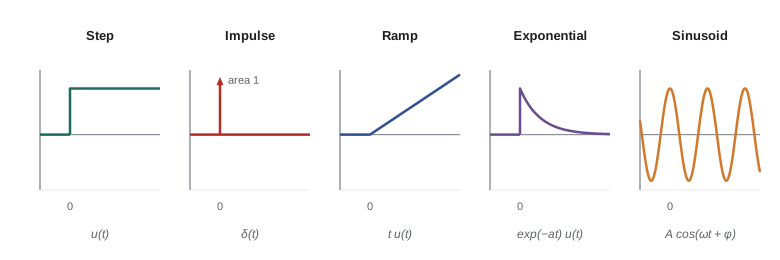
A handful of simple signals serve as building blocks and test inputs. Their value lies in the fact that complicated signals can be assembled from them, and that a system's response to one of them reveals its character.
The unit step \( u(t) \) is 0 for t < 0 and 1 for t ≥ 0. It models a sudden command, such as a set-point change from 0° to 30° (a step of height 30), or switching on a motor supply. The step response, studied in lesson 4, is the most common way to characterize a robot joint or a sensor.
The unit impulse \( \delta(t) \), also called the Dirac delta, is an idealized pulse of zero width, infinite height and unit area. It is not a function in the ordinary sense but is defined by what it does inside an integral: the sifting property
Physically, it represents any input that is short compared with the system's response time: a hammer tap on a robot arm during modal testing, a single kick of current, or a foot striking the ground. The impulse is the derivative of the step, and the step is the integral of the impulse. In discrete time the unit impulse \( \delta[n] \) is simply 1 at n = 0 and 0 elsewhere, with none of the subtleties.
The ramp \( r(t) = t\,u(t) \) models a constant-velocity command, such as a conveyor tracking task. The exponential \( e^{at}u(t) \) decays if a < 0 and grows if a > 0; exponentials are the natural responses of linear systems, and lesson 4 shows why. The sinusoid \( A\cos(\omega t + \phi) \) has amplitude A, angular frequency \( \omega = 2\pi f \) in radians per second and phase \( \phi \). Sinusoids are central because linear systems change only their amplitude and phase, which is the foundation of frequency response in lesson 7.
Euler's formula ties exponentials and sinusoids together:
Here j is the imaginary unit; engineers use j rather than i because i is already taken by current. The complex exponential \( e^{st} \) with \( s = \sigma + j\omega \) covers all the cases at once: a decaying or growing envelope set by \( \sigma \), oscillating at \( \omega \). Much of this course amounts to learning to think of signals as sums of such exponentials.
Worked problem
Describing a sinusoidal vibration
An accelerometer on a robot base records \( a(t) = 0.4\cos(150.8\,t + 0.5) \) m/s². Give the amplitude, frequency in hertz, period and phase in degrees.
Show solution
- Amplitude A = 0.4 m/s².
- Angular frequency \( \omega = 150.8 \) rad/s, so \( f = \omega/2\pi = 150.8/6.283 = 24.0 \) Hz.
- Period \( T_0 = 1/f = 41.7 \) ms.
- Phase \( 0.5 \) rad \( = 0.5 \times 180/\pi = 28.6° \).
Answer: A 24 Hz vibration of amplitude 0.4 m/s², period 41.7 ms, leading a pure cosine by 28.6°. A 24 Hz frequency suggests a rotating part turning at 24 revolutions per second, 1,440 rpm, worth checking against the motor and gearbox speeds.
Operations on signals
Three simple operations on the independent variable appear constantly. A time shift \( x(t - t_0) \) delays the signal by \( t_0 \) if \( t_0 > 0 \); sensor latency and communication delay are shifts. Time scaling \( x(at) \) compresses the signal if a > 1 and stretches it if a < 1, as when the same trajectory is replayed faster. Time reversal \( x(-t) \) flips the signal about t = 0, and it appears in the convolution integral of lesson 3. Amplitude operations, adding a constant offset or multiplying by a gain, model sensor bias and scale factor. Combinations need care with order: \( x(2t - 4) = x(2(t - 2)) \) is the signal compressed by two and then delayed by 2, not delayed by 4.
Signals are also added and multiplied. A measured signal is often modeled as the sum of a true value, a slowly varying bias and random noise: \( y(t) = x(t) + b(t) + v(t) \). Multiplying two signals, as a mixer or a modulator does, shifts frequencies, which is how radar and many communication links work.
Worked problem
Writing a command profile from standard signals
A joint is commanded to rest at 0 rad, ramp at 0.5 rad/s from t = 1 s to t = 3 s, and then hold. Write the command using steps and ramps.
Show solution
- A ramp starting at t = 1: \( 0.5\,(t - 1)\,u(t - 1) \).
- To stop the ramp at t = 3, subtract an identical ramp starting at t = 3: \( -0.5\,(t - 3)\,u(t - 3) \).
- For t > 3 the two cancel except for the constant \( 0.5 \times 2 = 1 \) rad.
Answer: \( \theta_{\text{cmd}}(t) = 0.5\,(t-1)\,u(t-1) - 0.5\,(t-3)\,u(t-3) \), which rises from 0 to 1 rad between 1 s and 3 s and then holds. Because the system is linear (lesson 2), its response to this command is the difference of two delayed ramp responses.
The size of a signal: energy and power
We often need a single number that says how big a signal is: to compare noise levels, set filter specifications or compute motor heating. Two measures are standard. The energy of a signal is
and its average power is the energy per unit time over a long interval:
The names come from electricity: if x is the voltage across a 1 Ω resistor, \( x^2 \) is the power dissipated. A pulse or a decaying transient has finite energy and zero average power; it is an energy signal. A sinusoid, a step or stationary noise has infinite energy but finite power; it is a power signal. The square root of the average power is the root-mean-square value, \( x_{\text{rms}} = \sqrt{P} \), the equivalent constant level that would deliver the same power. For a sinusoid of amplitude A, \( x_{\text{rms}} = A/\sqrt{2} \); for zero-mean noise the RMS value equals the standard deviation. Motor heating depends on RMS current, which is why ROB-220 sized motors by RMS torque.
Worked problem
Energy of a decaying transient
After an impact, a joint velocity error decays as \( e(t) = 0.2\,e^{-5t}u(t) \) rad/s. Find its energy.
Show solution
- \( E = \int_0^{\infty} 0.04\,e^{-10t}\,dt \).
- \( = 0.04 \times \left[-\tfrac{1}{10}e^{-10t}\right]_0^{\infty} = 0.04/10 \).
- \( E = 0.004 \) (rad/s)²·s.
Answer: The energy is 0.004 in units of (rad/s)²·s. Integral-of-squared-error measures like this are used to compare controller tunings: a smaller value means the disturbance was rejected more quickly or more gently.
Worked problem
RMS of a sensor signal
A current sensor reads a 2.0 A DC level plus a 0.6 A amplitude ripple at 20 kHz plus white noise with standard deviation 0.1 A. Find the RMS current.
Show solution
- Uncorrelated components add in power: \( P = 2.0^2 + (0.6/\sqrt{2})^2 + 0.1^2 \).
- \( = 4.0 + 0.18 + 0.01 = 4.19 \) A².
- \( I_{\text{rms}} = \sqrt{4.19} = 2.047 \) A.
Answer: About 2.05 A RMS. The ripple and noise add only 2 % to the RMS, but they matter for other reasons: the ripple frequency must be filtered before the ADC (lesson 9) and the noise limits the resolution of the current loop.
Signals in a robot: a worked inventory
It helps to see these categories applied. Consider a small mobile robot. Its wheel encoders produce discrete, quantized counts, sampled at 1 kHz. Its IMU delivers discrete samples of continuous accelerations and rates, each corrupted by bias and noise (ROB-220). Its lidar produces a periodic sequence of scans at 10 Hz, each a signal of angle. Its motor commands are discrete numbers converted to continuous voltages by PWM and filtered by the motor's own inductance. The battery voltage is a slowly varying continuous signal that sags with load. And its control software computes velocity from position by differencing samples, an operation whose effect on noise lesson 11 examines. Every one of these signals passes through systems, physical or computational, whose behavior the next eleven lessons will teach you to predict.
| Signal | Time | Amplitude | Typical rate | Main concern |
|---|---|---|---|---|
| Wheel encoder count | Discrete | Digital (integer) | 1 kHz | Quantization; differencing noise |
| IMU angular rate | Discrete samples of continuous | Digital, 16-bit | 200 Hz to 1 kHz | Bias, noise, aliasing |
| Motor current | Continuous, then sampled | Analog, then 12-bit | 10 to 40 kHz | PWM ripple, aliasing |
| Lidar scan | Discrete in angle and time | Digital ranges | 10 Hz scans | Latency, motion distortion |
| Battery voltage | Continuous | Analog | 10 Hz is plenty | Load-dependent sag |
| Joint position command | Discrete | Floating point | 100 Hz to 1 kHz | Smoothness; step changes |
import numpy as np
T, N = 0.001, 2000                 # 1 kHz for 2 s
t = np.arange(N) * T
x = 2.0 + 0.6*np.cos(2*np.pi*50*t)       # DC plus 50 Hz component
rng = np.random.default_rng(1)
y = x + rng.normal(0, 0.1, N)            # add white noise
print(f"mean      = {y.mean():.3f}")
print(f"RMS       = {np.sqrt(np.mean(y**2)):.3f}  (theory {np.sqrt(4 + 0.18 + 0.01):.3f})")
print(f"energy = {np.sum(y**2)*T:.2f} over 2 s (power signal: grows with duration)")mean = 1.999 RMS = 2.046 (theory 2.047) energy = 8.37 over 2 s (power signal: grows with duration)
The computed RMS agrees with the theory to within the scatter of a finite noise sample, and the energy keeps growing with the record length, confirming that this is a power signal rather than an energy signal.
Common mistakes
MistakeWriting x(n) and x[n] interchangeably
InsteadKeep parentheses for continuous time and square brackets for sample indices; the two need different mathematics.
MistakeConfusing hertz with radians per second
InsteadAlways convert with \( \omega = 2\pi f \); a 10 Hz signal has \( \omega \approx 62.8 \) rad/s.
MistakeTreating discrete time and digital as the same thing
InsteadSampling makes a signal discrete in time; quantization makes it digital in amplitude. They have different effects.
MistakeShifting before scaling in x(at − b)
InsteadFactor first: \( x(a(t - b/a)) \) is scaled by a and delayed by b/a.
MistakeAdding RMS values of independent components directly
InsteadAdd powers (squares of RMS values) and take the square root.
Summary and key terms
- A signal is a function of time, written x(t) for continuous time and x[n] for discrete time.
- Signals are classified as continuous or discrete, analog or digital, periodic or aperiodic, deterministic or random, and causal or non-causal.
- The step, impulse, ramp, exponential and sinusoid are standard building blocks and test inputs.
- The impulse is defined by its sifting property and models any input much shorter than the system response.
- Euler's formula links sinusoids and complex exponentials, which are the natural language of linear systems.
- Time shifting, scaling and reversal must be applied in the right order.
- Energy signals have finite energy; power signals have finite average power and an RMS value.
- Continuous-time signal
- A signal defined at every instant of time, written x(t).
- Discrete-time signal
- A signal defined only at sample indices, written x[n].
- Unit step
- A signal equal to 0 before t = 0 and 1 afterwards.
- Unit impulse
- An idealized pulse of zero width and unit area, defined by the sifting property.
- Sinusoid
- A signal of the form \( A\cos(\omega t + \phi) \).
- Angular frequency
- Frequency in radians per second, \( \omega = 2\pi f \).
- Periodic signal
- A signal that repeats exactly after a fundamental period.
- Energy
- The integral or sum of the squared magnitude of a signal.
- Average power
- Energy per unit time over a long interval.
- RMS value
- The square root of average power.
Practice problems
Work each problem on paper first, then reveal the answer to check.
Convert 1,200 rpm into hertz and radians per second.
Show answer
20 Hz; \( \omega = 125.7 \) rad/s.
A signal is \( 3\sin(40\pi t) \). What is its period?
Show answer
\( \omega = 40\pi \), f = 20 Hz, period 50 ms.
Write a pulse of height 2 lasting from t = 1 to t = 4 using unit steps.
Show answer
\( 2u(t-1) - 2u(t-4) \).
Evaluate \( \int \cos(t)\,\delta(t - \pi)\,dt \).
Show answer
By sifting, \( \cos\pi = -1 \).
What is the RMS value of a sinusoid with peak 10 V?
Show answer
\( 10/\sqrt{2} = 7.07 \) V.
Find the energy of \( x(t) = 3e^{-2t}u(t) \).
Show answer
\( 9/4 = 2.25 \).
Is a unit step an energy or a power signal? Find its average power.
Show answer
A power signal; average power 0.5 (it is 1 for half of a symmetric long interval).
Describe \( x(3t + 6) \) in terms of x(t).
Show answer
Compressed by 3 and advanced by 2: \( x(3(t + 2)) \).
A 12-bit ADC samples at 10 kHz. Is its output continuous or discrete, analog or digital?
Show answer
Discrete in time and digital in amplitude.
Noise of standard deviation 0.3 is added to a DC level of 4. What is the RMS of the sum?
Show answer
\( \sqrt{16 + 0.09} = 4.011 \).
Lesson quiz · 5 questions
Score 60% or more to complete this lesson.
Create a free account to save your progress, take quizzes and earn a certificate.