
ROB-230 · Lesson 12 of 12 · 34 min
State-space models and capstone: a motor-driven joint
Transfer functions describe how one input drives one output, and they hide everything that happens inside. Robots, however, have many inputs and outputs, internal variables that matter in their own right, such as motor current and link velocity, and initial conditions that cannot be ignored. The state-space model handles all of this. It writes a system as a set of first-order differential equations in matrix form, which is exactly the form that computers simulate, that modern control and estimation methods use (ROB-300 and ROB-310), and that extends naturally to many joints. This final lesson develops state-space models from the differential equations of earlier lessons, connects them to transfer functions through eigenvalues, discretizes them for implementation, and then pulls the whole course together in a capstone: modeling, analyzing, sampling and filtering a motor-driven robot joint.
State variables and the state-space form
The state of a system is the smallest set of variables that, together with future inputs, determines all future behavior. For a mass-spring-damper, position and velocity form the state: knowing both now, and the force from now on, fixes the motion forever. In general the number of state variables equals the order of the system, which is the number of independent energy stores: each inertia, spring, capacitor or inductor contributes one. A linear time-invariant system in state-space form is
where x is the state vector, u the input vector, y the output vector, and A, B, C and D constant matrices. A describes how the state evolves on its own, B how inputs push it, C which combinations are measured, and D any direct feedthrough from input to output, which is zero for most physical plants. For the mass-spring-damper with state \( \mathbf{x} = [x, \dot{x}]^T \), input force F and measured position,
The recipe is general: write each n-th order equation as n first-order equations by naming the derivatives as new states, then collect the coefficients into matrices.
Worked problem
State-space model of a DC motor driving a joint
A motor with inductance L, resistance R, constants \( k_t = k_e = k \), and total reflected inertia J with viscous friction b drives a joint. Choose states angle θ, speed ω and current i; input voltage v; output angle. Write A, B and C.
Show solution
- \( \dot{\theta} = \omega \).
- Mechanical: \( J\dot{\omega} = k\,i - b\,\omega \), so \( \dot{\omega} = (k/J)\,i - (b/J)\,\omega \).
- Electrical: \( L\,\dot{i} = v - R\,i - k\,\omega \), so \( \dot{i} = -(k/L)\,\omega - (R/L)\,i + v/L \).
- Collect: \( A = \begin{bmatrix} 0 & 1 & 0 \\ 0 & -b/J & k/J \\ 0 & -k/L & -R/L \end{bmatrix} \), \( B = \begin{bmatrix} 0 \\ 0 \\ 1/L \end{bmatrix} \), \( C = \begin{bmatrix} 1 & 0 & 0 \end{bmatrix} \).
Answer: A third-order model with three energy-related states: angle (the integrator), speed (kinetic energy in the inertia) and current (magnetic energy in the inductance). Unlike the transfer function, it exposes the current, which the controller must limit to protect the motor, and it can be simulated directly.
From state space to transfer function and back
Taking Laplace transforms with zero initial conditions, \( s\mathbf{X} = A\mathbf{X} + B\mathbf{U} \), so \( \mathbf{X} = (sI - A)^{-1}B\mathbf{U} \) and
The inverse \( (sI - A)^{-1} \) has the determinant \( \det(sI - A) \) as its denominator, so the poles of the transfer function are the roots of the characteristic polynomial \( \det(sI - A) = 0 \): the eigenvalues of A. Stability is therefore an eigenvalue question: the system is stable if all eigenvalues of A have negative real parts, or, in discrete time, if all eigenvalues of the discrete A lie inside the unit circle. Going the other way, any transfer function can be written in state-space form, but not uniquely: changing the choice of state variables by any invertible transformation gives a different A, B and C with the same input-output behavior and the same eigenvalues. Standard choices, such as the controllable canonical form, read the matrices directly off the transfer-function coefficients.
Worked problem
Eigenvalues and poles
For the mass-spring-damper with m = 0.5 kg, b = 4 N·s/m and k = 200 N/m (the camera mount of lesson 5), find the eigenvalues of A and confirm they match the transfer-function poles.
Show solution
- \( A = \begin{bmatrix} 0 & 1 \\ -400 & -8 \end{bmatrix} \).
- \( \det(sI - A) = s(s + 8) + 400 = s^2 + 8s + 400 \).
- Roots: \( s = -4 \pm j\sqrt{384} = -4 \pm 19.6j \).
Answer: The eigenvalues \( -4 \pm 19.6j \) are exactly the poles found in lesson 5 from the transfer function 2/(s² + 8s + 400). The two descriptions are equivalent for input-output behavior; state space simply keeps the internal velocity visible.
Solving and simulating state equations
The state equation has an explicit solution. With no input, \( \mathbf{x}(t) = e^{At}\mathbf{x}(0) \), where the matrix exponential \( e^{At} = I + At + (At)^2/2! + \cdots \) generalizes the scalar exponential of first-order systems. With an input, the solution adds a convolution of the input with \( e^{At}B \), the matrix version of lesson 3. In practice we rarely evaluate these formulas by hand. Instead we discretize. If the input is held constant over each sample period T, as it is behind a zero-order hold (lesson 9), the exact discrete model is
This is the zero-order-hold discretization of lesson 10 in matrix form: each eigenvalue \( \lambda \) of A becomes an eigenvalue \( e^{\lambda T} \) of \( A_d \). The discrete model is what runs inside a simulator, a model-predictive controller or a Kalman filter. A convenient trick computes both matrices at once from a single matrix exponential of an augmented matrix, as the code below does. Forward Euler, \( A_d \approx I + AT \), \( B_d \approx BT \), is simpler but, as lesson 10 warned, can be inaccurate or unstable for stiff systems, such as a motor whose electrical time constant is much shorter than its mechanical one.
import numpy as np
def expm(M, terms=30):                  # matrix exponential by scaling and squaring
    n = max(0, int(np.ceil(np.log2(max(np.abs(M).sum(axis=1).max(), 1e-12)))) + 1)
    Ms = M / 2**n; E = np.eye(M.shape[0]); term = np.eye(M.shape[0])
    for k in range(1, terms):
        term = term @ Ms / k; E = E + term
    for _ in range(n): E = E @ E
    return E
k, R, L, J, b = 0.05, 1.0, 0.5e-3, 2e-4, 1e-5     # motor and joint parameters
A = np.array([[0, 1, 0], [0, -b/J, k/J], [0, -k/L, -R/L]])
B = np.array([[0], [0], [1/L]])
print("eigenvalues of A:", np.round(np.sort(np.linalg.eigvals(A).real), 1))
T = 1e-3
M = np.zeros((4, 4)); M[:3, :3] = A*T; M[:3, 3:] = B*T
E = expm(M); Ad, Bd = E[:3, :3], E[:3, 3:]
print("eigenvalues of Ad (exact):", np.round(np.sort(np.linalg.eigvals(Ad).real), 4))
print("eigenvalues of I + A*T (Euler):", np.round(np.sort(np.linalg.eigvals(np.eye(3) + A*T).real), 4))eigenvalues of A: [-1987.4 -12.6 0. ] eigenvalues of Ad (exact): [0.137 0.9874 1. ] eigenvalues of I + A*T (Euler): [-0.9874 0.9874 1. ]
The continuous model has an integrator pole at zero, a mechanical pole and a very fast electrical pole near −2,000 rad/s. Exact discretization maps them all safely inside the unit circle. Forward Euler maps the fast electrical pole to a negative value of magnitude near one, giving a barely stable, sign-alternating mode that does not exist in the real motor. That is exactly the failure lesson 10 predicted for aT near 2.
Capstone: modeling and filtering a motor-driven joint
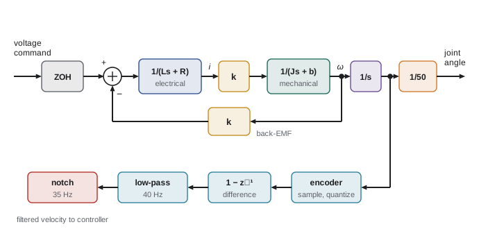
The final task brings the course together. A small collaborative arm's elbow joint is driven through a 50:1 gearbox by a DC motor; a 4,096-count encoder on the motor shaft measures position, sampled at 1 kHz, and a current sensor is sampled at 20 kHz. The arm's first structural mode is at 35 Hz. We need a model for control design, a sampling and filtering plan, and an estimate of the velocity signal quality. The parameters are \( k = 0.05 \) N·m/A, \( R = 1.0 \) Ω, \( L = 0.5 \) mH, motor-side reflected inertia \( J = 2 \times 10^{-4} \) kg·m² including the link, and negligible friction.
Worked problem
Capstone step 1: time constants and model order
Find the electrical and mechanical time constants and decide whether the inductance can be neglected for position control at a 10 Hz bandwidth.
Show solution
- Electrical: \( \tau_e = L/R = 0.5 \) ms (pole at −2,000 rad/s, about 320 Hz).
- Mechanical: \( \tau_m = JR/k^2 = 2 \times 10^{-4} \times 1/0.0025 = 0.08 \) s (pole at −12.5 rad/s).
- The electrical pole is about 30 times above the 10 Hz (63 rad/s) bandwidth, so for position-loop design it adds only a few degrees of phase lag.
Answer: τ_e = 0.5 ms and τ_m = 80 ms. A second-order model (integrator plus mechanical pole) is adequate for designing the 10 Hz position loop, with the electrical pole kept in the simulation for checking. The current loop, which must be much faster, needs the full model.
Worked problem
Capstone step 2: sampling and anti-aliasing
Check the 1 kHz position sampling against the 10 Hz loop bandwidth, and specify the analog filter for the 20 kHz current sampling if the PWM frequency is 25 kHz.
Show solution
- Position loop: 1 kHz is 100 times the bandwidth. Delay of ZOH plus one sample of computation is 1.5 ms; at a 10 Hz crossover that costs \( 360 \times 10 \times 0.0015 = 5.4° \). Acceptable.
- Current sampling: Nyquist is 10 kHz, and 25 kHz PWM ripple would alias to \( |25 - 20| = 5 \) kHz.
- Better: synchronize current sampling with the PWM so each sample is taken at the midpoint of the PWM period, where the ripple crosses its average, and add an RC filter at about 5 kHz to suppress switching spikes.
Answer: Position sampling at 1 kHz is comfortable. For current, PWM-synchronized sampling is the standard fix, because it samples the ripple at the same phase every period and so measures its average; an anti-aliasing RC filter near 5 kHz handles the residual spikes.
Worked problem
Capstone step 3: velocity estimate and notch
Velocity is estimated by differencing the motor encoder at 1 kHz and low-pass filtering at 40 Hz. Estimate the raw and filtered velocity noise at the motor and at the joint, and choose a notch for the 35 Hz mode.
Show solution
- From lesson 9, raw differenced noise is \( \sqrt{2}\,q/(\sqrt{12}\,T) \) with \( q = 2\pi/4096 \): 0.627 rad/s at the motor.
- A first-order low-pass filter reduces white noise by roughly \( \sqrt{\pi f_c/f_s} \) for \( f_c \ll f_s \) (its equivalent noise bandwidth is \( \pi f_c/2 \) out of a Nyquist band of \( f_s/2 \)): \( \sqrt{\pi \times 40/1000} = 0.354 \), giving about 0.22 rad/s.
- At the joint, divide by the gear ratio: 0.0044 rad/s, about 0.25 °/s.
- Notch at 35 Hz with Q = 3 (width about 12 Hz, allowing for payload shifts); phase cost at a 10 Hz crossover \( \approx -\arctan\left(\frac{(35/3)(10)}{35^2 - 10^2}\right) = -\arctan(0.104) = -5.9° \).
Answer: Filtered joint velocity noise is about 0.25 °/s, ample for a cobot elbow. The 40 Hz low-pass costs about \( \arctan(10/40) = 14° \) at crossover and the notch about 6°, so with sampling delay the measurement chain uses roughly 25° of phase budget, leaving room for a design with 50° or more of phase margin. These numbers become the starting point for the controller design in ROB-300.
| Item | Value | Course tool used |
|---|---|---|
| Electrical / mechanical time constants | 0.5 ms / 80 ms | First-order models (lesson 4) |
| Model for position-loop design | Integrator plus mechanical pole | Transfer functions, state space (lessons 5, 12) |
| Position sampling | 1 kHz, 5.4° delay cost at 10 Hz | Zero-order hold (lesson 9) |
| Current sampling | 20 kHz synchronized to 25 kHz PWM | Aliasing (lesson 9) |
| Velocity estimate | Difference plus 40 Hz low-pass, about 0.25 °/s noise at joint | Digital filters (lesson 11) |
| Resonance treatment | Notch at 35 Hz, Q = 3 | Notch filters, Bode phase (lessons 7, 11) |
| Phase budget of measurement chain | About 25° at 10 Hz | Frequency response (lesson 7) |
The capstone shows how the topics of this course interlock. Differential equations and state space give the model; transfer functions and Bode plots show where its poles and resonances lie; the sampling theorem and the zero-order hold set the update rates; aliasing dictates how current is measured; and digital filters, budgeted in phase, turn raw encoder counts into usable velocity. The same reasoning applies to every axis of every robot, from a hobby rover to a surgical arm.
Common mistakes
MistakeChoosing more state variables than energy stores
InsteadThe number of states equals the system order; redundant states make A singular in misleading ways.
MistakeForgetting D when a system has direct feedthrough
InsteadInclude D for systems such as sensors with instantaneous response components.
MistakeDiscretizing a stiff model with forward Euler
InsteadUse exact zero-order-hold discretization, especially when electrical and mechanical time constants differ widely.
MistakeAssuming a state-space model is unique
InsteadAny invertible change of state variables gives an equivalent model with the same eigenvalues.
MistakeDesigning a filter chain without a phase budget
InsteadAdd up sampling, computation and filter phase lag at crossover before tuning the controller.
Summary and key terms
- The state is the minimal set of variables that, with future inputs, determines future behavior; its size equals the system order.
- State-space models write a system as ẋ = Ax + Bu, y = Cx + Du and handle many inputs, outputs and internal variables.
- The transfer function is C(sI − A)⁻¹B + D, and its poles are the eigenvalues of A.
- Stability requires eigenvalues of A in the left half-plane, or of \( A_d \) inside the unit circle.
- Exact zero-order-hold discretization gives \( A_d = e^{AT} \) and maps each eigenvalue λ to \( e^{\lambda T} \).
- Forward Euler can mis-map fast eigenvalues of stiff models.
- Modeling, sampling, aliasing, filtering and phase budgeting combine into a complete measurement design for a robot joint.
- State
- The minimal set of variables that summarizes a system's past.
- State vector
- The column vector x of state variables.
- State-space model
- The matrix equations ẋ = Ax + Bu, y = Cx + Du.
- System matrix
- The matrix A, which governs the unforced evolution of the state.
- Input matrix
- The matrix B, which maps inputs into state derivatives.
- Output matrix
- The matrix C, which maps states to outputs.
- Eigenvalue
- A value λ with Av = λv; the eigenvalues of A are the poles.
- Matrix exponential
- The series \( e^{At} = I + At + (At)^2/2! + \cdots \).
- Stiff system
- A system with time constants that differ by orders of magnitude.
- Phase budget
- An accounting of all phase lag in a loop at its crossover frequency.
Practice problems
Work each problem on paper first, then reveal the answer to check.
How many states does a two-mass, two-spring system have?
Show answer
Four (a position and a velocity for each mass).
Write A for \( \ddot{y} + 3\dot{y} + 2y = u \) with state [y, ẏ].
Show answer
\( \begin{bmatrix} 0 & 1 \\ -2 & -3 \end{bmatrix} \).
Find the eigenvalues of that A.
Show answer
−1 and −2.
Is a system with eigenvalues −3, 0.5 and −10 stable?
Show answer
No; the eigenvalue 0.5 is positive.
A continuous eigenvalue of −100 is sampled at T = 5 ms by exact discretization. Where does it go?
Show answer
\( e^{-0.5} = 0.607 \).
Where would forward Euler put that eigenvalue?
Show answer
\( 1 - 0.5 = 0.5 \).
What D is appropriate for a motor model from voltage to angle?
Show answer
D = 0; there is no instantaneous feedthrough.
A motor has L = 2 mH and R = 0.5 Ω. What is its electrical time constant?
Show answer
4 ms.
A 30:1 gearbox follows a motor-side velocity estimate with 0.3 rad/s noise. What is the joint-side noise?
Show answer
0.01 rad/s.
List three contributors to a joint loop's phase budget.
Show answer
Zero-order hold and computation delay, sensor filters, notch filters (also the plant's neglected fast poles).
Lesson quiz · 5 questions
Score 60% or more to complete this lesson.
Create a free account to save your progress, take quizzes and earn a certificate.