Lagrangian dynamics of manipulators

The Newton–Euler approach of lesson 1 treats each link separately and tracks the forces between them. For understanding and for control design it is often easier to work with energy. The Lagrangian method describes the whole robot by two scalar functions, its kinetic and potential energy, written in terms of the joint angles, and produces the equations of motion by differentiation alone. Constraint forces inside the joints never appear, because they do no work. The result is the standard manipulator equation, \( \mathbf{M}(\mathbf{q})\ddot{\mathbf{q}} + \mathbf{C}(\mathbf{q},\dot{\mathbf{q}})\dot{\mathbf{q}} + \mathbf{g}(\mathbf{q}) = \boldsymbol{\tau} \), whose structure every model-based controller in this course exploits. This lesson derives it for a pendulum and for a two-link planar arm, explains each term physically and lists the properties that make it tractable.

Generalized coordinates and the Lagrangian

A manipulator with n joints has n degrees of freedom, and the joint variables \( \mathbf{q} = [q_1, \ldots, q_n]^{\mathsf{T}} \), angles for revolute joints and displacements for prismatic ones, are a natural set of generalized coordinates: knowing them fixes the position of every point on the robot through forward kinematics. The Lagrangian is the difference between kinetic and potential energy,

and the equations of motion follow from the Euler–Lagrange equations, one for each coordinate:

Here \( \tau_i \) is the generalized force for coordinate i: the joint torque for a revolute joint or the joint force for a prismatic one, plus any other non-conservative forces such as friction projected onto that coordinate. The recipe is mechanical: write the position of each link's center of mass in terms of q, differentiate to get velocities, assemble T and V, and apply the formula. It never requires free-body diagrams of the joints.

A first example: the pendulum joint

Apply the method to the single link of lesson 1, with joint angle q measured from the horizontal, inertia I about the joint and center of mass at distance \( l_c \). The kinetic energy is \( T = \tfrac{1}{2}I\dot{q}^2 \) and the potential energy, taking zero height at the joint, is \( V = mgl_c\sin q \).

Kinetic energy of a manipulator and the inertia matrix

For a chain of links, each link's center-of-mass velocity and angular velocity are linear in the joint rates, related through the link Jacobians of ROB-210: \( \mathbf{v}_{ci} = \mathbf{J}_{vi}(\mathbf{q})\dot{\mathbf{q}} \) and \( \boldsymbol{\omega}_i = \mathbf{J}_{\omega i}(\mathbf{q})\dot{\mathbf{q}} \). Substituting into the rigid-body kinetic energy and summing over links gives a quadratic form in the joint rates:

The n × n matrix \( \mathbf{M}(\mathbf{q}) \) is the manipulator inertia matrix, also called the mass matrix. Its diagonal entry \( M_{ii} \) is the inertia felt by joint i when only that joint moves; its off-diagonal entries describe inertial coupling, the torque one joint must apply when another accelerates. Because kinetic energy is positive for any motion, M is symmetric and positive definite in every configuration.

The two-link planar arm

The two-link planar arm moving in a vertical plane is the standard teaching example, because it shows every term of the general equation while remaining small enough to write out. Link 1 has length \( l_1 \), mass \( m_1 \), center of mass at distance \( l_{c1} \) from joint 1 and inertia \( I_1 \) about its own center of mass; link 2 has \( l_2, m_2, l_{c2}, I_2 \). The angle \( q_1 \) is measured from the horizontal and \( q_2 \) is the elbow angle relative to link 1, as in ROB-210.

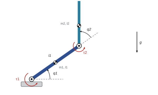
Working through the kinetic and potential energies (the center of mass of link 2 is at \( l_1(\cos q_1, \sin q_1) + l_{c2}(\cos(q_1 + q_2), \sin(q_1 + q_2)) \)) and applying the Euler–Lagrange equations gives, with the shorthand \( c_2 = \cos q_2 \), \( s_2 = \sin q_2 \) and \( c_{12} = \cos(q_1 + q_2) \):

Three constants \( \alpha, \beta, \delta \) capture all the inertial parameters. The inertia felt by the shoulder, \( \alpha + 2\beta\cos q_2 \), is largest when the elbow is straight (\( q_2 = 0 \)) and smallest when it is folded, so the same shoulder motor sees a load that varies by a factor of two or more as the elbow moves.

Interpreting the Coriolis, centrifugal and gravity terms

The vector \( \mathbf{C}(\mathbf{q},\dot{\mathbf{q}})\dot{\mathbf{q}} \) collects velocity-product torques. Terms in a single squared rate, such as \( \beta s_2\dot{q}_1^2 \) at the elbow, are centrifugal: when the shoulder swings quickly, link 2 is flung outward and the elbow must resist it. Terms in a product of two different rates, such as \( -2\beta s_2\dot{q}_1\dot{q}_2 \) at the shoulder, are Coriolis torques that arise when one joint's motion changes the moment arm of another link's moving mass. These terms grow with the square of speed, so they matter for fast robots and fade at low speed. The gravity vector \( \mathbf{g}(\mathbf{q}) \) depends only on configuration; it is the torque each joint needs to hold the arm still, and the first term in the shoulder entry includes the weight of link 2 acting at the elbow.

The manipulator equation and its properties

For any serial manipulator, rigid links and ideal joints, the Euler–Lagrange equations produce the same structure:

Friction, actuator dynamics and contact forces are added to this core model in later lessons. Its properties are what make robot control theory possible:

• M(q) is symmetric and positive definite, so it is always invertible: \( \ddot{\mathbf{q}} = \mathbf{M}^{-1}(\boldsymbol{\tau} - \mathbf{C}\dot{\mathbf{q}} - \mathbf{g}) \), the forward dynamics used in simulation.
• M(q) is bounded above and below for revolute arms, so the inertia never becomes zero or infinite.
• With C defined through Christoffel symbols, the matrix \( \dot{\mathbf{M}} - 2\mathbf{C} \) is skew-symmetric. Physically this expresses energy conservation: the Coriolis and centrifugal forces do no net work. It is the key step in stability proofs for many robot controllers.
• The dynamics are linear in a set of inertial parameters (masses, first moments, inertias), so \( \mathbf{M}\ddot{\mathbf{q}} + \mathbf{C}\dot{\mathbf{q}} + \mathbf{g} = \mathbf{Y}(\mathbf{q},\dot{\mathbf{q}},\ddot{\mathbf{q}})\boldsymbol{\theta} \). This makes parameter identification a least-squares problem and underpins adaptive control (lesson 11).

The Christoffel definition gives each element of C as \( C_{kj} = \sum_i \tfrac{1}{2}\left(\frac{\partial M_{kj}}{\partial q_i} + \frac{\partial M_{ki}}{\partial q_j} - \frac{\partial M_{ij}}{\partial q_k}\right)\dot{q}_i \). For the two-link arm it yields \( \mathbf{C} = \beta s_2\begin{bmatrix} -\dot{q}_2 & -(\dot{q}_1 + \dot{q}_2) \\ \dot{q}_1 & 0 \end{bmatrix} \), which reproduces the vector given earlier.

Forward dynamics and simulation

Inverse dynamics computes the torque for a desired motion; forward dynamics computes the motion produced by given torques by solving the manipulator equation for \( \ddot{\mathbf{q}} \) and integrating. The code below implements both for the two-link arm. It first computes the torque needed to hold a configuration, then releases the arm with zero torque and integrates the motion with a fourth-order Runge–Kutta step, checking that total energy is conserved, a standard test that a dynamic model has been coded correctly.

import numpy as np
m1, m2, l1, lc1, lc2, I1, I2, g = 3, 2, 0.4, 0.2, 0.15, 0.04, 0.015, 9.81
a = I1 + I2 + m1*lc1**2 + m2*(l1**2 + lc2**2); b = m2*l1*lc2; d = I2 + m2*lc2**2
def M(q):  return np.array([[a + 2*b*np.cos(q[1]), d + b*np.cos(q[1])], [d + b*np.cos(q[1]), d]])
def Cqd(q, qd):
    s = np.sin(q[1]); return np.array([-b*s*(2*qd[0]*qd[1] + qd[1]**2), b*s*qd[0]**2])
def G(q):
    c1, c12 = np.cos(q[0]), np.cos(q[0] + q[1])
    return np.array([(m1*lc1 + m2*l1)*g*c1 + m2*lc2*g*c12, m2*lc2*g*c12])
def energy(q, qd):
    V = (m1*lc1 + m2*l1)*g*np.sin(q[0]) + m2*lc2*g*np.sin(q[0] + q[1])
    return 0.5*qd @ M(q) @ qd + V
q0 = np.array([0.0, np.pi/2])
print("holding torque (N m):", np.round(G(q0), 3))
def f(x, tau):
    q, qd = x[:2], x[2:]
    qdd = np.linalg.solve(M(q), tau - Cqd(q, qd) - G(q))
    return np.concatenate([qd, qdd])
x, h = np.array([0.0, 0.3, 0.0, 0.0]), 1e-3
E0 = energy(x[:2], x[2:])
for k in range(2000):                    # 2 s with zero torque (arm falls freely)
    k1 = f(x, 0); k2 = f(x + h/2*k1, 0); k3 = f(x + h/2*k2, 0); k4 = f(x + h*k3, 0)
    x = x + h/6*(k1 + 2*k2 + 2*k3 + k4)
print("q after 2 s (rad):", np.round(x[:2], 3))
print(f"energy drift: {energy(x[:2], x[2:]) - E0:.2e} J")

holding torque (N m): [13.734  0.   ]
q after 2 s (rad): [-1.848 -0.156]
energy drift: -8.51e-09 J

The holding torques match the hand calculation, and with no friction or input the total energy stays constant to within about 10⁻⁸ J over two seconds of chaotic double-pendulum motion. A drift of joules would signal an error in M, C or g, or a time step that is too large.

Scaling up: real robots

A six-axis industrial arm has a 6 × 6 inertia matrix whose entries are long trigonometric expressions in all six angles. Nobody writes them out by hand. Robotics libraries build the model from a URDF or similar description and compute inverse dynamics with the recursive Newton–Euler algorithm, forward dynamics with the articulated-body algorithm, and the inertia matrix itself with the composite rigid-body algorithm, all in time roughly proportional to the number of links. The value of the Lagrangian derivation is conceptual: it reveals the structure, symmetric positive-definite inertia, velocity-squared coupling, configuration-dependent gravity and linearity in parameters, that controllers exploit regardless of how the numbers are computed. Model parameters from CAD are usually refined by identification experiments in which the robot follows exciting trajectories while joint torques are measured, and the parameter vector is found by least squares using the linear-in-parameters property.