Trajectory generation and time scaling

A controller tracks a reference; the quality of that reference largely decides how well the robot moves. If the reference jumps from one position to another, the controller sees a huge error, demands torques the motors cannot deliver, saturates, winds up and overshoots, as lesson 4 showed. If instead the reference moves smoothly, with velocity and acceleration the actuators can supply, the controller only has to correct small deviations, and model-based feedforward (lesson 9) can supply nearly all the torque in advance. Trajectory generation turns a list of goals, 'move joint 2 from 0.3 to 1.2 rad', 'pass through these via points', 'arrive at this pose with zero velocity', into time functions \( q_d(t), \dot{q}_d(t), \ddot{q}_d(t) \) that respect limits on velocity, acceleration, jerk and torque. This lesson covers polynomial trajectories, trapezoidal and jerk-limited velocity profiles, multi-joint synchronization, via points and time scaling.

Path and trajectory

A path is a geometric curve, the set of configurations the robot passes through, without timing. A trajectory is a path with a time law attached. Separating the two is useful: a path can be written as \( \mathbf{q}(s) \) for a path parameter s running from 0 to 1, and a time scaling s(t) then decides how fast the robot moves along it. For a straight line in joint space from \( \mathbf{q}_0 \) to \( \mathbf{q}_f \), \( \mathbf{q}(s) = \mathbf{q}_0 + s(\mathbf{q}_f - \mathbf{q}_0) \), and all joints start and stop together. Velocities and accelerations follow by the chain rule: \( \dot{\mathbf{q}} = \mathbf{q}'(s)\dot{s} \) and \( \ddot{\mathbf{q}} = \mathbf{q}'(s)\ddot{s} + \mathbf{q}''(s)\dot{s}^2 \). Choosing s(t) well is most of the work.

Cubic polynomial trajectories

The simplest smooth time scaling is a cubic polynomial, \( q(t) = a_0 + a_1t + a_2t^2 + a_3t^3 \), whose four coefficients can satisfy four boundary conditions: position and velocity at the start and at the end. For a rest-to-rest move from \( q_0 \) to \( q_f \) in time T, with \( \Delta = q_f - q_0 \):

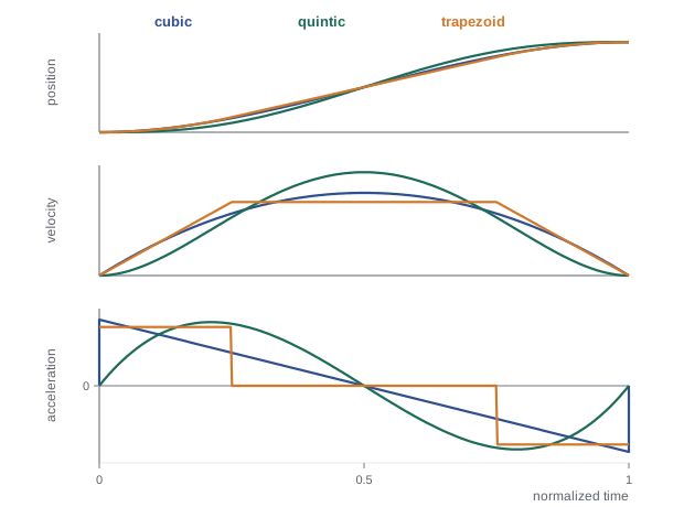
Velocity is a parabola peaking at mid-move at \( 1.5\Delta/T \); acceleration falls linearly from \( 6\Delta/T^2 \) at the start to \( -6\Delta/T^2 \) at the end. The weakness is that acceleration jumps from zero to \( 6\Delta/T^2 \) at the start and from \( -6\Delta/T^2 \) to zero at the end. These jumps mean infinite jerk, which excites structural vibration, a problem for flexible joints and for robots carrying liquids or delicate parts.

Quintic polynomials

A fifth-order polynomial has six coefficients, enough to fix position, velocity and acceleration at both ends. For rest-to-rest motion with zero boundary accelerations, written with the normalized time \( \sigma = t/T \):

Acceleration now starts and ends at zero, so jerk is finite and the motion is much smoother. The price is higher peaks for the same duration: peak velocity \( 1.875\Delta/T \) and peak acceleration \( 10\Delta/(\sqrt{3}T^2) \approx 5.77\Delta/T^2 \), occurring at \( \sigma = 0.5 \mp 0.289 \). Quintic profiles are standard for smooth point-to-point moves, and in general form, with nonzero boundary velocities and accelerations, they join segments smoothly.

Trapezoidal velocity profiles

Industrial motion controllers mostly use trapezoidal velocity profiles: accelerate at a constant rate \( a_{\max} \), cruise at \( v_{\max} \), decelerate at \( a_{\max} \). Each phase uses the actuator fully, so for given velocity and acceleration limits the trapezoid gives the minimum time among profiles that respect those limits. The acceleration time is \( t_a = v_{\max}/a_{\max} \), and the distance covered while accelerating and decelerating together is \( v_{\max}^2/a_{\max} \). If the move is longer than this, the profile has a cruise phase and the total time is

If the move is shorter, the joint never reaches \( v_{\max} \); the profile becomes a triangle with peak velocity \( \sqrt{\Delta a_{\max}} \) and total time \( 2\sqrt{\Delta/a_{\max}} \).

Jerk-limited (S-curve) profiles

The trapezoid's acceleration jumps instantly between 0 and \( \pm a_{\max} \), with infinite jerk at four instants, which excites vibration much like the cubic's end jumps. Jerk-limited profiles, often called S-curves, ramp the acceleration up and down at a maximum jerk \( j_{\max} \), giving seven phases: jerk up, constant acceleration, jerk down, cruise, and the mirror image. Each acceleration ramp takes \( a_{\max}/j_{\max} \), and the total time increases by about that much over the trapezoid. A useful rule from vibration theory: if the acceleration ramp time equals the period of a structural mode, the profile excites that mode very little. Commercial motion controllers expose jerk as a parameter for this reason.

Synchronizing joints

For a multi-joint move, each joint could follow its own minimum-time profile, but then they finish at different times and the tool follows an odd curve. Usually all joints are synchronized: find the move time each joint would need on its own, take the longest, and slow the others to match. With a common normalized time scaling s(t), every joint follows \( q_i(t) = q_{0i} + \Delta_i s(t) \), so the robot moves in a straight line in joint space and all joints start and stop together. The slowest joint, the one with the longest individual time, is called the limiting or leading joint.

Via points and splines

Many tasks need the robot to pass through intermediate points without stopping: around an obstacle, along a weld seam, through a sequence of camera viewpoints. Stopping at each via point wastes time and causes jerky motion. Instead, a spline joins polynomial segments so that position, velocity and acceleration are continuous at each via point. A natural cubic spline through N points has continuous acceleration and is found by solving a tridiagonal linear system for the velocities at the via points; quintic splines also make jerk continuous. Industrial controllers often use blending instead: each straight segment is followed until close to the via point, then a parabolic or polynomial blend rounds the corner, with a programmable blend radius that trades accuracy at the via point against speed.

Joint space versus Cartesian space

Everything above works in joint space, which is simple and naturally respects joint limits, but the tool path between endpoints is a curve that depends on the robot's geometry. Many tasks, such as inserting a peg, welding a seam or moving through a narrow gap, require the tool to follow a straight line or a specified curve in Cartesian space. Then the path is defined in task space, for example \( \mathbf{x}(s) = \mathbf{x}_0 + s(\mathbf{x}_f - \mathbf{x}_0) \) for position with spherical linear interpolation (slerp, ROB-210) for orientation, and inverse kinematics (ROB-210) converts each point to joint angles. Cartesian paths can pass near singularities, where joint velocities become very large for modest tool speed, so the time scaling must be slowed there or the path changed.

Time scaling under torque limits

Velocity and acceleration limits are proxies; the true limits are the motor torques, which depend on the dynamics of lessons 2 and 3. For a fixed path, the manipulator equation can be written in terms of s, and the torque required becomes \( \boldsymbol{\tau} = \mathbf{m}(s)\ddot{s} + \mathbf{c}(s)\dot{s}^2 + \mathbf{g}(s) \). Each joint's torque limit then bounds \( \ddot{s} \) as a function of s and \( \dot{s} \). Time-optimal path parameterization algorithms find the fastest s(t) that keeps every joint inside its torque limit at every point, giving bang-bang behavior where at least one joint is always at its limit. A simpler, widely used approach is uniform time scaling: plan a trajectory, check the torques with inverse dynamics, and if any exceed the limit, stretch the duration. Stretching time by a factor k divides velocities by k and accelerations by \( k^2 \), so inertial and velocity-product torques fall by \( k^2 \) while gravity is unchanged.

import numpy as np
def cubic(sig):  return 3*sig**2 - 2*sig**3, 6*sig - 6*sig**2, 6 - 12*sig
def quintic(sig):
    return (10*sig**3 - 15*sig**4 + 6*sig**5, 30*sig**2 - 60*sig**3 + 30*sig**4,
            60*sig - 180*sig**2 + 120*sig**3)
D, T = 1.2, 1.5
sig = np.linspace(0, 1, 100001)
for name, f in (("cubic", cubic), ("quintic", quintic)):
    p, v, a = f(sig)
    print(f"{name:8s}: v_peak = {D/T*v.max():.3f} rad/s, a_peak = {D/T**2*abs(a).max():.3f} rad/s^2, "
          f"a(0) = {D/T**2*a[0]:.2f}")
def trapezoid_time(D, vmax, amax):
    D = abs(D)
    return D/vmax + vmax/amax if D >= vmax**2/amax else 2*np.sqrt(D/amax)
times = [trapezoid_time(d, 2.0, 8.0) for d in (1.2, 0.3, -0.8)]
print("trapezoid times (s):", np.round(times, 3), "-> synchronized T =", round(max(times), 3))

cubic   : v_peak = 1.200 rad/s, a_peak = 3.200 rad/s^2, a(0) = 3.20
quintic : v_peak = 1.500 rad/s, a_peak = 3.079 rad/s^2, a(0) = 0.00
trapezoid times (s): [0.85  0.387 0.65 ] -> synchronized T = 0.85

The numbers confirm the formulas: the quintic peaks at 1.5 rad/s and about 3.08 rad/s² but starts with zero acceleration, while the cubic starts with a jump to 3.2 rad/s². The synchronized trapezoid time is set by the 1.2 rad joint.