Uncertainty in robotics and probability review

A robot never knows exactly where it is. Its wheels slip, its encoders count in discrete ticks, its lidar returns are corrupted by dust and glass, its GNSS fix wanders by meters under trees, and the world itself changes as people walk past and doors open and close. A robot that ignores this uncertainty and trusts a single best guess will eventually drive into a wall when that guess turns out to be wrong. Probabilistic robotics takes the opposite view: the robot keeps track not of one estimate but of a probability distribution over everything it might need to know, updates that distribution as it moves and senses, and makes decisions that account for how confident it is. This course develops the tools that make this possible, from the Bayes filter through Kalman and particle filters to factor-graph smoothing, and ends with a complete localization design. This first lesson sets out where uncertainty comes from and reviews the probability that every later lesson uses.

Where uncertainty comes from

It helps to separate the sources of uncertainty, because each is handled differently. Sensor noise is the random scatter in measurements: a lidar range that reads 4.02 m, then 3.98 m, then 4.01 m for the same wall. Sensor limitations are systematic: a sonar cannot see a thin chair leg, a camera is blind in the dark, GNSS fails indoors. Actuation uncertainty comes from the gap between commanded and actual motion: a wheel commanded to turn 1 radian may turn 0.98 radians because of slip, backlash or uneven floors. Model uncertainty arises because every model of a robot or its environment is an approximation, from the assumed wheel radius to the map of the building. Finally, the world is dynamic: furniture moves, people appear, lighting changes. A probabilistic estimator models all of these as random variables with distributions, and its output is a belief, a distribution that summarizes what the robot knows.

The payoff is robustness. A robot that knows its position estimate has a standard deviation of 2 cm can safely pass through a doorway 10 cm wider than itself; one whose uncertainty has grown to 30 cm should slow down, look for landmarks, or ask for help. Probabilistic estimates also let a robot combine sensors sensibly: a precise but occasionally wrong sensor and a noisy but reliable one can be weighted according to their known uncertainties, so that the combination is better than either alone.

Random variables and distributions

A random variable X is a quantity whose value is uncertain, described by a probability distribution. For a discrete variable, such as which of ten corridor cells the robot is in, the distribution is a probability mass function p(x) with \( \sum_x p(x) = 1 \). For a continuous variable, such as the robot's x coordinate, it is a probability density function p(x) with \( \int p(x)\,dx = 1 \); probabilities come from integrating the density over an interval, and the density itself can exceed 1. Two summaries matter most. The mean or expected value is

and the variance, which measures spread, is

The standard deviation σ has the same units as X and is the number engineers usually quote: 'the position is known to about 3 cm'. Expectation is linear, so \( E[aX + b] = aE[X] + b \), and variance scales with the square of a constant, \( \text{Var}(aX + b) = a^2\text{Var}(X) \). These two rules, applied to vectors, give the prediction step of the Kalman filter.

The Gaussian distribution

The Gaussian, or normal, distribution is the workhorse of estimation. In one dimension its density is

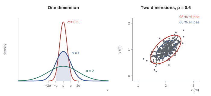
written \( X \sim \mathcal{N}(\mu, \sigma^2) \). About 68 % of the probability lies within one standard deviation of the mean, 95.4 % within two and 99.7 % within three, figures worth memorizing because they turn a reported σ into an intuitive range. Gaussians are popular for three reasons. Many physical noise sources are approximately Gaussian, because they are the sum of many small independent effects (the central limit theorem). A Gaussian is completely described by its mean and variance, so an estimator only has to track two numbers per variable. And Gaussians stay Gaussian under linear transformations and when combined by Bayes' rule with Gaussian measurements, which is exactly why the Kalman filter is exact for linear systems. Their weakness is that they are unimodal: a Gaussian cannot represent 'the robot is either at the north door or the south door', which is why lessons 2 and 8 introduce histogram and particle representations.

Multivariate Gaussians and covariance

A robot's state is a vector, such as \( \mathbf{x} = [x, y, \theta]^{\mathsf{T}} \) for a planar mobile robot. The multivariate Gaussian generalizes the bell curve:

The covariance matrix Σ is symmetric and positive definite. Its diagonal entries are the variances of each component; the off-diagonal entry \( \Sigma_{ij} = E[(x_i - \mu_i)(x_j - \mu_j)] \) is the covariance between components i and j. Dividing by the standard deviations gives the correlation coefficient \( \rho_{ij} = \Sigma_{ij}/(\sigma_i\sigma_j) \), between −1 and 1. Correlation matters enormously in robotics: after a robot drives forward while slightly uncertain about its heading, its sideways position error is strongly correlated with its heading error, because a heading error is what caused the sideways drift. A filter that ignored that correlation would make poor use of a later heading measurement, which should also correct the sideways position.

Surfaces of constant density are ellipsoids, \( (\mathbf{x} - \boldsymbol{\mu})^{\mathsf{T}}\boldsymbol{\Sigma}^{-1}(\mathbf{x} - \boldsymbol{\mu}) = c \). The quantity on the left is the squared Mahalanobis distance, the distance from the mean measured in standard deviations along each principal direction; it reappears in lesson 9 for rejecting outlier measurements. In two dimensions, the ellipse axes point along the eigenvectors of Σ and have half-lengths \( \sqrt{c\lambda_i} \), where \( \lambda_i \) are the eigenvalues. For two dimensions, the ellipse with c = 5.99 contains 95 % of the probability, and c = 2.30 contains about 68 %.

Joint, marginal and conditional probability

Three operations on distributions are used constantly. The joint distribution p(x, y) gives the probability of both values together. The marginal distribution of x is obtained by summing or integrating out the other variable, \( p(x) = \int p(x, y)\,dy \); this is the law of total probability, and it is exactly what the prediction step of every filter does when it integrates over the previous state. The conditional distribution of x given that y is known is

so that \( p(x, y) = p(x \mid y)p(y) \). Two variables are independent when \( p(x, y) = p(x)p(y) \), meaning knowing y tells you nothing about x. They are conditionally independent given z when \( p(x, y \mid z) = p(x \mid z)p(y \mid z) \). Conditional independence, not full independence, is the assumption that makes robot estimation tractable: two lidar readings taken from the same pose are not independent (both depend on where the robot is), but given the pose they can often be treated as independent, because their remaining errors come from separate noise. For Gaussians, marginalizing simply means dropping rows and columns of the mean and covariance, and conditioning has a closed form that the Kalman update uses.

Bayes' rule

Rearranging the definition of conditional probability gives Bayes' rule, the engine of all probabilistic estimation:

Here x is something the robot wants to know, such as its position, and z is a measurement. The prior p(x) is the belief before the measurement. The likelihood p(z | x) is the sensor model: how probable this measurement would be if the state were x. The posterior p(x | z) is the updated belief. The denominator p(z) does not depend on x and is usually written as a normalizer η, computed at the end by making the posterior sum or integrate to 1. The beauty of Bayes' rule is that it inverts the direction of reasoning: sensor manufacturers and engineers can describe p(z | x), how a sensor responds to a known world, and Bayes' rule turns that into p(x | z), what the world is likely to be given the reading.

import numpy as np
rng = np.random.default_rng(7)
# a 2-D position estimate: sample it and check the sample statistics
mu = np.array([2.0, 1.0])
S = np.array([[0.05, 0.03], [0.03, 0.05]])
X = rng.multivariate_normal(mu, S, size=20000)
print("sample mean:", np.round(X.mean(axis=0), 3))
print("sample covariance:\n", np.round(np.cov(X.T), 4))
# fraction inside the 95 % ellipse (squared Mahalanobis distance < 5.99)
d = X - mu
m2 = np.einsum('ij,jk,ik->i', d, np.linalg.inv(S), d)
print(f"inside 95 % ellipse: {np.mean(m2 < 5.99):.3f}")
lam, V = np.linalg.eigh(S)
print("semi-axes of 95 % ellipse (m):", np.round(np.sqrt(5.99*lam), 3))

sample mean: [2.003 1.002]
sample covariance:
 [[0.05   0.0299]
 [0.0299 0.0494]]
inside 95 % ellipse: 0.950
semi-axes of 95 % ellipse (m): [0.346 0.692]

The sample statistics reproduce the mean and covariance, and almost exactly 95 % of the samples fall inside the ellipse with squared Mahalanobis distance below 5.99, confirming the ellipse semi-axes found by hand. Simulations like this one, with a seeded random number generator so that results are reproducible, are the standard way to check estimation code: if a filter claims a 95 % ellipse, roughly 95 % of the true states in a simulation should lie inside it.

Notation for the rest of the course

The course uses the notation of the probabilistic robotics literature. The state at time t is \( x_t \), the control applied between t − 1 and t is \( u_t \), and the measurement taken at time t is \( z_t \). The sequence of all measurements up to time t is written \( z_{1:t} \). The belief is the posterior over the current state given all data, \( bel(x_t) = p(x_t \mid z_{1:t}, u_{1:t}) \), and the predicted belief before incorporating the latest measurement is \( \overline{bel}(x_t) = p(x_t \mid z_{1:t-1}, u_{1:t}) \). Two models describe the robot and its sensors: the motion model \( p(x_t \mid x_{t-1}, u_t) \), covered in lesson 3, and the measurement model \( p(z_t \mid x_t) \), covered in lesson 4. Every filter in this course is a particular way of representing beliefs and computing them from these two models.