The extended Kalman filter

Robots are not linear. A differential-drive robot moves along arcs governed by sines and cosines of its heading, and a landmark sensor measures ranges with square roots and bearings with arctangents. Pass a Gaussian through such functions and the result is no longer Gaussian, so the Kalman filter's exactness is lost. The extended Kalman filter, EKF, keeps the Kalman structure by linearizing the motion and measurement functions around the current estimate at every step. It is an approximation, and it can fail, but when uncertainty is small relative to the curvature of the functions it works remarkably well. The EKF navigated aircraft and spacecraft for decades and is still the default estimator in drone autopilots and many robot localization stacks. This lesson derives the EKF, applies it to landmark-based localization and examines the conditions under which it breaks down.

Linearization

A nonlinear function g can be approximated near a point by its first-order Taylor expansion, \( g(\mathbf{x}) \approx g(\boldsymbol{\mu}) + \mathbf{G}(\mathbf{x} - \boldsymbol{\mu}) \), where the Jacobian \( \mathbf{G} = \partial g/\partial \mathbf{x} \) is evaluated at μ. A linear function of a Gaussian is Gaussian, so the approximation yields a Gaussian with mean \( g(\boldsymbol{\mu}) \) and covariance \( \mathbf{G}\boldsymbol{\Sigma}\mathbf{G}^{\mathsf{T}} \). The approximation is good when the function is nearly straight over the region where the belief has most of its probability, roughly μ ± 2σ. A robot whose heading is known to within 1° sees almost no curvature in \( \cos\theta \); one whose heading is uncertain by 60° sees a great deal.

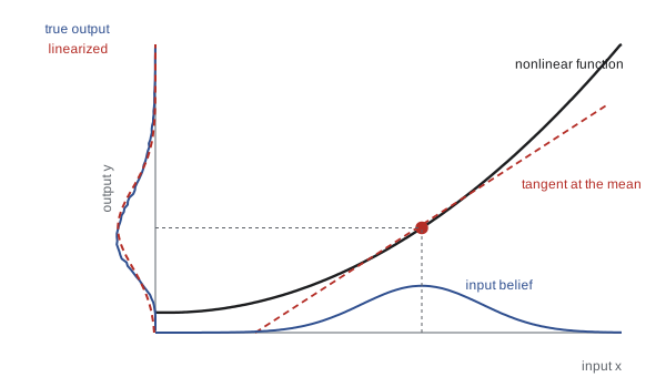
The EKF equations

With motion model \( \mathbf{x}_t = g(\mathbf{x}_{t-1}, \mathbf{u}_t) + \mathbf{w}_t \) and measurement model \( \mathbf{z}_t = h(\mathbf{x}_t) + \mathbf{v}_t \), the EKF replaces A and H in the Kalman filter by Jacobians evaluated at the latest estimate:

Here \( \mathbf{G}_t = \partial g/\partial\mathbf{x} \) at \( \boldsymbol{\mu}_{t-1} \) and \( \mathbf{H}_t = \partial h/\partial\mathbf{x} \) at \( \bar{\boldsymbol{\mu}}_t \). Note what is and is not linearized: the means are propagated through the true nonlinear functions g and h, while only the covariances use the Jacobians. When the noise enters through the controls, as in the motion models of lesson 3, the process noise becomes \( \mathbf{Q}_t = \mathbf{V}_t\mathbf{M}_t\mathbf{V}_t^{\mathsf{T}} \), mapping the control-noise covariance M into state space with the control Jacobian V. Computationally the EKF costs about the same as a Kalman filter, roughly cubic in the state dimension, which for a three-dimensional pose is trivial.

EKF localization with known landmarks

Consider a planar robot with state \( [x, y, \theta]^{\mathsf{T}} \), odometry inputs of a forward distance d and a turn δ per step, and a sensor that measures range and bearing to landmarks with known positions and identities. The motion model and its Jacobians come straight from lesson 3, the measurement model and its Jacobian from lesson 4. The EKF loop is: predict with each odometry step; for each landmark observed, compute the expected range and bearing from the predicted pose, form the innovation (with the bearing wrapped), compute H for that landmark and apply the update. Multiple landmarks seen at the same time can be processed one after another, or stacked into one larger measurement vector; with independent noise the result is the same.

import numpy as np
rng = np.random.default_rng(21)
LM = np.array([[5.0, 5.0], [-4.0, 6.0], [2.0, -5.0]])       # known landmarks
def wrap(a): return (a + np.pi) % (2*np.pi) - np.pi
def g(x, u): d, dth = u; return np.array([x[0] + d*np.cos(x[2]), x[1] + d*np.sin(x[2]), wrap(x[2] + dth)])
def h(x, m): dx, dy = m - x[:2]; return np.array([np.hypot(dx, dy), wrap(np.arctan2(dy, dx) - x[2])])
M = np.diag([0.02**2, np.radians(1)**2]); R = np.diag([0.1**2, np.radians(2)**2])
x = np.array([0.0, 0.0, 0.0]); mu = x.copy(); S = np.diag([0.01, 0.01, 0.001])
errs = []
for t in range(200):
    u = (0.1, 0.05)                                              # drive in a circle
    x = g(x, (u[0] + rng.normal(0, 0.02), u[1] + rng.normal(0, np.radians(1))))
    th = mu[2]; d = u[0]
    G = np.array([[1, 0, -d*np.sin(th)], [0, 1, d*np.cos(th)], [0, 0, 1]])
    V = np.array([[np.cos(th), 0], [np.sin(th), 0], [0, 1]])
    mu = g(mu, u); S = G @ S @ G.T + V @ M @ V.T
    for m in LM:
        z = h(x, m) + rng.multivariate_normal([0, 0], R)
        dx, dy = m - mu[:2]; q = dx*dx + dy*dy; r = np.sqrt(q)
        H = np.array([[-dx/r, -dy/r, 0], [dy/q, -dx/q, -1]])
        y = z - h(mu, m); y[1] = wrap(y[1])
        K = S @ H.T @ np.linalg.inv(H @ S @ H.T + R)
        mu = mu + K @ y; mu[2] = wrap(mu[2]); S = (np.eye(3) - K @ H) @ S
    errs.append(np.r_[x[:2] - mu[:2], wrap(x[2] - mu[2])])
e = np.array(errs)
print("RMSE x, y (m):", np.round(np.sqrt((e[:, :2]**2).mean(0)), 3), " heading (deg):", round(np.degrees(np.sqrt((e[:, 2]**2).mean())), 2))
print("final 1-sigma (m, m, deg):", np.round(np.sqrt(np.diag(S))[:2], 3), round(np.degrees(np.sqrt(S[2, 2])), 2))

RMSE x, y (m): [0.027 0.021]  heading (deg): 0.87
final 1-sigma (m, m, deg): [0.035 0.017] 0.87

With three landmarks always in view, the EKF holds the pose to a few centimeters and a fraction of a degree, and the reported standard deviations are of the same size as the actual errors, a sign of a well-matched filter. Remove the landmarks and the covariance would grow without bound as odometry drift accumulates, exactly as dead reckoning does; add them back and the filter pulls the estimate in and shrinks the covariance in a single update.

When the EKF fails

The EKF's linearization introduces two kinds of error. The first is bias in the mean: the mean of a nonlinear function is not the function of the mean, so the EKF's predicted mean can be systematically wrong, as the banana example of lesson 3 showed. The second is error in the covariance: the Jacobian captures only the local slope, so when curvature matters the true spread is larger or differently shaped than \( \mathbf{G}\boldsymbol{\Sigma}\mathbf{G}^{\mathsf{T}} \). Both grow with the size of the uncertainty relative to the scale over which the functions curve. A particularly dangerous consequence is inconsistency: the EKF can become overconfident, its covariance shrinking faster than its actual error, after which it ignores the very measurements that could rescue it. Linearizing about a wrong estimate makes this worse, because the Jacobians themselves are then wrong.

The EKF also inherits the Kalman filter's unimodal belief. It cannot represent 'I am at one of these three doors', so it cannot perform global localization from an unknown start, and it handles data association errors badly: a single wrong landmark match pulls the estimate firmly in the wrong direction. Practical remedies include initializing carefully (from a known start or a global method), gating measurements whose innovation is implausible (lesson 9), inflating Q to stay humble, and, for strongly nonlinear measurements, the iterated EKF, which re-linearizes the measurement function around the updated estimate and repeats the update a few times, equivalent to Gauss–Newton optimization of the posterior.

A simple diagnostic catches many EKF problems before they reach the field. Log the NIS of every landmark update. If the EKF is consistent, the NIS values for 2-D range-bearing updates should average about 2, and about 99 % of them should fall below 9.21. A slow upward trend in NIS while the reported covariance keeps shrinking is the signature of creeping overconfidence, and it usually appears long before the position error becomes visible on a map.

Two refinements are common in modern robotics. The error-state EKF, used in most inertial navigation and visual-inertial odometry systems, estimates a small error around a nominal trajectory rather than the full state; small errors keep linearization accurate and make it natural to handle orientations, which do not form a vector space, with a three-element rotation error. And for orientations in general, filters now often work on the rotation group directly (sometimes called Lie-group or invariant EKFs), avoiding the singularities of Euler angles discussed in ROB-210.