Analysis of variance and experimental design

Lesson 8 compared two groups. Experiments often compare more: four fertilizer formulations, five incubation temperatures, three diets crossed with two strains of mice. Running a t test for every pair inflates the false positive rate and ignores the structure of the design. The analysis of variance (ANOVA), developed by R. A. Fisher at the Rothamsted agricultural research station in the 1920s alongside the principles of randomization and blocking, compares several means in one analysis by partitioning the total variation in the data into parts attributable to different sources. This final lesson covers one-way ANOVA, follow-up comparisons, two-way designs with interaction, randomized blocks, the control of multiple comparisons, and an end-to-end example that draws the course together.

The idea of ANOVA

Suppose k groups are compared, with H₀: μ₁ = μ₂ = … = μ_k. If H₀ is true, the group means should differ only by about as much as random variation within groups would produce. ANOVA compares two estimates of variance. The between-group mean square measures how much the group means vary around the grand mean; the within-group mean square measures how much observations vary around their own group means. Their ratio is the F statistic.

If H₀ is true, both mean squares estimate σ² and F is near 1. If the group means really differ, the between-group mean square is inflated and F is large. Under H₀ and the usual assumptions, F follows an F distribution with k − 1 and N − k degrees of freedom, where N is the total number of observations. The total sum of squares splits exactly into between and within parts, SS_total = SS_between + SS_within, which is why the method is called the analysis of variance.

One-way ANOVA

import numpy as np
from scipy import stats
rng = np.random.default_rng(1529)

# Invented: dry biomass (g) of wheat seedlings under four nitrogen treatments, 8 pots each
groups = {"control": rng.normal(4.0, 0.8, 8), "low N": rng.normal(4.6, 0.8, 8),
          "medium N": rng.normal(5.5, 0.8, 8), "high N": rng.normal(5.7, 0.8, 8)}
data = list(groups.values())
y = np.concatenate(data); N, k = y.size, len(data)
grand = y.mean()
ss_b = sum(g.size*(g.mean() - grand)**2 for g in data)
ss_w = sum(np.sum((g - g.mean())**2) for g in data)
ms_b, ms_w = ss_b/(k - 1), ss_w/(N - k)
F = ms_b/ms_w
print(f"{'source':9s} {'df':>3s} {'SS':>8s} {'MS':>8s} {'F':>7s}")
print(f"{'between':9s} {k-1:3d} {ss_b:8.3f} {ms_b:8.3f} {F:7.2f}")
print(f"{'within':9s} {N-k:3d} {ss_w:8.3f} {ms_w:8.3f}")
print(f"{'total':9s} {N-1:3d} {ss_b + ss_w:8.3f}")
print(f"p = {stats.f.sf(F, k-1, N-k):.2g}; scipy f_oneway gives F = {stats.f_oneway(*data).statistic:.2f}")
print(f"eta squared = SS_between/SS_total = {ss_b/(ss_b + ss_w):.2f}")
for name, g in groups.items():
    print(f"  {name:9s} mean = {g.mean():.2f} g")

source     df       SS       MS       F
between     3   12.316    4.105    8.02
within     28   14.339    0.512
total      31   26.654
p = 0.00052; scipy f_oneway gives F = 8.02
eta squared = SS_between/SS_total = 0.46
  control   mean = 4.16 g
  low N     mean = 4.96 g
  medium N  mean = 5.60 g
  high N    mean = 5.72 g

The ANOVA table summarizes the partition. η² (eta squared), the proportion of total variation explained by the treatments, is the ANOVA counterpart of R². ANOVA is in fact a special case of regression with indicator variables for the groups, so everything in lessons 10 and 11 about residuals and assumptions applies.

The assumptions are independence (from randomization and proper replication), approximately normal residuals, and similar variances across groups. One-way ANOVA is fairly robust to non-normality with moderate, equal group sizes, and to unequal variances when group sizes are equal. When variances differ and sizes are unequal, Welch’s ANOVA is the safer choice, as Welch’s t test was for two groups. The rank-based Kruskal–Wallis test (stats.kruskal) is the nonparametric alternative.

Follow-up comparisons

A significant F test says that not all means are equal but not which ones differ. Comparing every pair of k groups involves k(k − 1)/2 comparisons, six for four groups, and testing each at α = 0.05 raises the chance of at least one false positive well above 5 percent. Tukey’s honestly significant difference (HSD) procedure compares all pairs while holding the family-wise error rate, the probability of any false positive among the comparisons, at α. When a few specific comparisons were planned in advance, such as each treatment against the control, more powerful methods such as Dunnett’s test, or a small number of pre-specified contrasts, are appropriate.

import numpy as np
from scipy import stats
rng = np.random.default_rng(1529)
names = ["control", "low N", "medium N", "high N"]
data = [rng.normal(m, 0.8, 8) for m in (4.0, 4.6, 5.5, 5.7)]   # same data as above
res = stats.tukey_hsd(*data)
ci = res.confidence_interval(0.95)
for i in range(4):
    for j in range(i + 1, 4):
        print(f"{names[j]:8s} - {names[i]:8s}: diff = {data[j].mean() - data[i].mean():5.2f}, "
              f"95% CI {-ci.high[i, j]:5.2f} to {-ci.low[i, j]:5.2f}, adj. p = {res.pvalue[i, j]:.3f}")

low N    - control : diff =  0.80, 95% CI -0.18 to  1.78, adj. p = 0.137
medium N - control : diff =  1.44, 95% CI  0.47 to  2.42, adj. p = 0.002
high N   - control : diff =  1.56, 95% CI  0.58 to  2.54, adj. p = 0.001
medium N - low N   : diff =  0.64, 95% CI -0.33 to  1.62, adj. p = 0.296
high N   - low N   : diff =  0.76, 95% CI -0.22 to  1.73, adj. p = 0.173
high N   - medium N: diff =  0.11, 95% CI -0.86 to  1.09, adj. p = 0.989

Two-way ANOVA and interaction

A factorial experiment crosses two or more factors, so that every combination of levels is tested. Factorial designs are efficient, because every observation contributes information about every factor, and they are the only way to detect interactions, where the effect of one factor depends on the level of another. A two-way ANOVA partitions the variation into the main effect of factor A, the main effect of factor B, the A × B interaction, and the residual.

The invented experiment below crosses two watering regimes with three nitrogen levels, with five pots per combination. In a balanced design like this, the sums of squares can be computed directly from the cell, row and column means.

import numpy as np
from scipy import stats
rng = np.random.default_rng(1530)

# Invented 2 x 3 factorial: water (dry, wet) x nitrogen (0, 50, 100 kg/ha), 5 pots per cell
cell_means = np.array([[3.0, 3.6, 3.8],      # dry: nitrogen helps a little
                       [3.4, 5.0, 6.4]])     # wet: nitrogen helps a lot
r = 5
y = cell_means[:, :, None] + rng.normal(0, 0.6, (2, 3, r))
a, b = y.shape[0], y.shape[1]
grand = y.mean()
mA, mB, mAB = y.mean(axis=(1, 2)), y.mean(axis=(0, 2)), y.mean(axis=2)
ss_A = b*r*np.sum((mA - grand)**2)
ss_B = a*r*np.sum((mB - grand)**2)
ss_AB = r*np.sum((mAB - mA[:, None] - mB[None, :] + grand)**2)
ss_E = np.sum((y - mAB[:, :, None])**2)
df = {"water": a - 1, "nitrogen": b - 1, "water x N": (a - 1)*(b - 1), "residual": a*b*(r - 1)}
ss = {"water": ss_A, "nitrogen": ss_B, "water x N": ss_AB, "residual": ss_E}
ms_E = ss_E/df["residual"]
for src in ("water", "nitrogen", "water x N"):
    F = ss[src]/df[src]/ms_E
    print(f"{src:10s} df = {df[src]}, SS = {ss[src]:6.2f}, F = {F:6.2f}, p = {stats.f.sf(F, df[src], df['residual']):.2g}")
print(f"{'residual':10s} df = {df['residual']}, SS = {ss_E:6.2f}, MS = {ms_E:.3f}")
print("cell means (rows dry, wet; columns N 0, 50, 100):")
print(np.round(mAB, 2))

water      df = 1, SS =  12.39, F =  32.66, p = 6.9e-06
nitrogen   df = 2, SS =  22.37, F =  29.49, p = 3.4e-07
water x N  df = 2, SS =   2.75, F =   3.63, p = 0.042
residual   df = 24, SS =   9.10, MS = 0.379
cell means (rows dry, wet; columns N 0, 50, 100):
[[2.79 3.7  4.17]
 [3.4  4.87 6.24]]

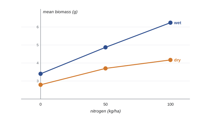
The significant interaction means that the effect of nitrogen cannot be described by a single number: it is small when water is limited and large when it is plentiful. Main effects should then be interpreted with caution, and results presented as cell means or simple effects within each level of the other factor. An interaction plot, with one line per level of one factor, makes this visible: parallel lines indicate no interaction, diverging or crossing lines indicate interaction.

Randomized block designs

Lesson 1 introduced blocking: grouping similar experimental units and randomizing treatments within each block. In agriculture, blocks are often strips of a field that differ in soil; in the laboratory, they may be days, batches of reagent or litters of animals. The analysis removes the block-to-block variation from the residual, which can greatly increase precision. A randomized complete block design with one observation per treatment per block is analyzed as a two-way ANOVA without interaction, with blocks as the second factor.

import numpy as np
from scipy import stats
rng = np.random.default_rng(1531)

# Invented: yield (t/ha) of 4 varieties in 6 field blocks with a strong fertility gradient
t, blk = 4, 6
variety = np.array([0.0, 0.3, 0.6, 0.4])
block = np.linspace(-1.5, 1.5, blk)
y = 5 + variety[:, None] + block[None, :] + rng.normal(0, 0.25, (t, blk))

grand = y.mean()
ss_T = blk*np.sum((y.mean(axis=1) - grand)**2)
ss_B = t*np.sum((y.mean(axis=0) - grand)**2)
ss_tot = np.sum((y - grand)**2)
ss_E = ss_tot - ss_T - ss_B
df_T, df_B, df_E = t - 1, blk - 1, (t - 1)*(blk - 1)
F_block = (ss_T/df_T)/(ss_E/df_E)
p_block = stats.f.sf(F_block, df_T, df_E)
F_one = stats.f_oneway(*y)                      # ignoring blocks (wrong for this design)
print(f"with blocks:    F(varieties) = {F_block:.2f} on {df_T} and {df_E} df, p = {p_block:.2g}")
print(f"ignoring blocks: F(varieties) = {F_one.statistic:.2f} on {df_T} and {t*blk - t} df, p = {F_one.pvalue:.2g}")
print(f"share of total SS due to blocks = {ss_B/ss_tot:.0%}")

with blocks:    F(varieties) = 5.32 on 3 and 15 df, p = 0.011
ignoring blocks: F(varieties) = 0.33 on 3 and 20 df, p = 0.8
share of total SS due to blocks = 91%

Ignoring the blocks leaves the large fertility gradient in the residual, swamping the variety differences; accounting for them reveals the differences clearly. Blocking must be planned in the design and reflected in the analysis; it cannot be added afterwards if treatments were not randomized within blocks.

Multiple comparisons beyond ANOVA

The problem of multiple testing extends far beyond pairwise comparisons. A study that measures 20 outcomes, or a genomics experiment that tests 20,000 genes, will produce false positives by chance alone. Two broad strategies exist. Controlling the family-wise error rate (FWER) limits the chance of any false positive. The Bonferroni correction tests each of m hypotheses at α/m; it is simple and always valid but conservative. The Holm procedure is uniformly more powerful: sort the p-values, compare the smallest with α/m, the next with α/(m − 1), and so on, stopping at the first that fails. Controlling the false discovery rate (FDR), the expected proportion of false positives among the rejected hypotheses, is less strict and more appropriate for large screening studies. The Benjamini–Hochberg procedure, published in 1995, is the standard method.

import numpy as np
from scipy import stats

p = np.array([0.001, 0.004, 0.012, 0.019, 0.030, 0.041, 0.090, 0.220, 0.510, 0.740])
m, alpha = p.size, 0.05
order = np.argsort(p)

bonf = p < alpha/m
holm = np.zeros(m, bool)
for rank, i in enumerate(order):
    if p[i] < alpha/(m - rank): holm[i] = True
    else: break
bh = stats.false_discovery_control(p, method="bh") < alpha

print("p-value  unadjusted  Bonferroni  Holm  BH")
for i in range(m):
    print(f"{p[i]:7.3f}  {str(p[i] < alpha):>10s}  {str(bonf[i]):>10s}  {str(holm[i]):>4s}  {str(bh[i]):>4s}")
print(f"rejections: unadjusted {np.sum(p < alpha)}, Bonferroni {bonf.sum()}, Holm {holm.sum()}, BH {bh.sum()}")

p-value  unadjusted  Bonferroni  Holm  BH
  0.001        True        True  True  True
  0.004        True        True  True  True
  0.012        True       False  False  True
  0.019        True       False  False  True
  0.030        True       False  False  False
  0.041        True       False  False  False
  0.090       False       False  False  False
  0.220       False       False  False  False
  0.510       False       False  False  False
  0.740       False       False  False  False
rejections: unadjusted 6, Bonferroni 2, Holm 2, BH 4

Which strategy is right depends on the consequences of a false positive. For a few confirmatory comparisons that will each be acted upon, FWER control is appropriate. For screening thousands of candidates that will be followed up in further experiments, FDR control is more sensible. The worst practice is to test many hypotheses, report only the significant ones, and make no adjustment, sometimes called p-hacking or the garden of forking paths.

Putting it all together: an end-to-end study

The final example follows one invented study from question to report, drawing on every lesson. A research group wants to know whether a commercial biochar soil amendment increases the growth of canola seedlings, and whether any effect depends on the soil type.

import numpy as np
from scipy import stats
rng = np.random.default_rng(1532)

# Invented data: 3 biochar rates x 2 soils x 6 benches (blocks), one pot per combination per bench
rates, soils, benches = [0, 2, 5], ["sandy", "clay loam"], 6
true = np.array([[2.0, 2.5, 2.9],      # sandy: biochar helps
                 [2.6, 2.7, 2.6]])     # clay loam: little effect
bench = rng.normal(0, 0.3, benches)
y = true[:, :, None] + bench[None, None, :] + rng.normal(0, 0.45, (2, 3, benches))

a, b, r = y.shape
grand = y.mean()
mS, mR, mSR, mK = y.mean(axis=(1, 2)), y.mean(axis=(0, 2)), y.mean(axis=2), y.mean(axis=(0, 1))
ss = {"soil": b*r*np.sum((mS - grand)**2), "biochar": a*r*np.sum((mR - grand)**2),
      "soil x biochar": r*np.sum((mSR - mS[:, None] - mR[None, :] + grand)**2),
      "bench (block)": a*b*np.sum((mK - grand)**2)}
ss_E = np.sum((y - grand)**2) - sum(ss.values())
df = {"soil": a - 1, "biochar": b - 1, "soil x biochar": (a - 1)*(b - 1), "bench (block)": r - 1}
df_E = a*b*r - 1 - sum(df.values())
ms_E = ss_E/df_E
for src in ss:
    F = ss[src]/df[src]/ms_E
    print(f"{src:15s} df = {df[src]}, F = {F:6.2f}, p = {stats.f.sf(F, df[src], df_E):.2g}")
print(f"residual        df = {df_E}, MS = {ms_E:.3f}")

# Planned contrasts: each biochar rate vs none, within each soil (4 contrasts), Holm-adjusted
se = np.sqrt(2*ms_E/r)
tcrit_df = df_E
pvals, rows = [], []
for i, soil in enumerate(soils):
    for j in (1, 2):
        d = mSR[i, j] - mSR[i, 0]
        t = d/se
        pvals.append(2*stats.t.sf(abs(t), tcrit_df)); rows.append((soil, rates[j], d))
pvals = np.array(pvals)
order = np.argsort(pvals); m = len(pvals); adj = np.empty(m); running = 0.0
for rank, k in enumerate(order):
    running = max(running, min(1.0, (m - rank)*pvals[k])); adj[k] = running
tq = stats.t.ppf(1 - 0.05/(2*m), tcrit_df)       # Bonferroni-width intervals (conservative)
for (soil, rate, d), pa in zip(rows, adj):
    print(f"{soil:9s} {rate}% vs 0%: diff = {d:5.2f} g, simultaneous 95% CI {d - tq*se:5.2f} to {d + tq*se:5.2f}, Holm p = {pa:.3f}")

soil            df = 1, F =   0.11, p = 0.75
biochar         df = 2, F =   5.88, p = 0.0081
soil x biochar  df = 2, F =   4.52, p = 0.021
bench (block)   df = 5, F =   5.18, p = 0.0021
residual        df = 25, MS = 0.162
sandy     2% vs 0%: diff =  0.36 g, simultaneous 95% CI -0.27 to  0.98, Holm p = 0.413
sandy     5% vs 0%: diff =  1.04 g, simultaneous 95% CI  0.41 to  1.66, Holm p = 0.001
clay loam 2% vs 0%: diff =  0.07 g, simultaneous 95% CI -0.56 to  0.69, Holm p = 1.000
clay loam 5% vs 0%: diff =  0.08 g, simultaneous 95% CI -0.55 to  0.70, Holm p = 1.000

The analysis tells a clear story. In sandy soil, the 5 percent rate increases seedling biomass by about 1 g, an effect whose simultaneous interval excludes zero; the 2 percent rate gives a smaller gain that the experiment cannot distinguish from zero. In clay loam, which already holds water well, biochar has little effect at either rate. This difference between soils is the soil × biochar interaction. The bench blocks absorb a substantial part of the variation, sharpening the comparisons. The residual SD in the experiment (√0.162 ≈ 0.40 g) turned out larger than the 0.3 g assumed in planning, so the realized power was lower than intended, one reason the 2 percent effect remains uncertain. Honest reporting says so, and a follow-up study could use more benches. A report would present the interaction plot and the four contrasts with their simultaneous intervals, and discuss the practical meaning of the gain in sandy soil.

Reproducibility and research integrity

Statistics serves science only when the work can be checked. Reproducible analysis means that another researcher, given the data and code, obtains the same numbers. That requires scripts rather than manual spreadsheet steps, recorded random seeds (as in every simulation in this course), documented software versions, and data that are archived with clear metadata. Pre-registration of hypotheses, outcomes and analyses, already standard for clinical trials, separates confirmatory tests from exploratory findings and protects against the forking paths described above. Replication by independent groups remains the ultimate test of any result.

Research involving human participants in the United States must also follow the Federal Policy for the Protection of Human Subjects (the Common Rule), which requires review by an institutional review board, informed consent and protection of privacy. Animal research is overseen by institutional animal care and use committees under the Animal Welfare Act and Public Health Service policy. Statistical design is part of ethics: an underpowered study exposes participants or animals to risk without a realistic chance of answering its question, and an oversized one uses more than necessary.

Where next? STAT-251 develops probability theory in more depth, and STAT-252 provides the mathematical foundations of estimation and testing that underlie the methods in this course. Courses in specific fields extend them: generalized linear models for counts and binary outcomes, mixed models for repeated and clustered measurements, survival analysis, time series, and Bayesian methods, which make the reasoning of lesson 3 the basis for all inference.