
STAT-151 · Lesson 8 of 12 · 27 min
Comparing two groups: t tests and nonparametric alternatives
Many experiments compare two conditions: treated and control plots, before and after an intervention, two populations of a species, two analytical methods. This lesson covers the main tools for comparing two groups on a numerical outcome. The key distinction is between independent samples, where different units are measured in each group, and paired samples, where the same or matched units are measured twice. Choosing the wrong analysis for the design is one of the most common errors in scientific papers. The lesson also covers the assumptions of t tests, how to check them, and the rank-based nonparametric alternatives for data that violate them.
Paired designs
In a paired design each observation in one group has a natural partner in the other: the same patient before and after treatment, the left and right leaves of the same plant, two methods applied to the same water sample. Pairing removes the variation between units, which is often large, and so can make comparisons much more precise. The analysis reduces to a one-sample problem: compute the difference for each pair, then apply the one-sample t procedures of lessons 6 and 7 to the differences.
Here d̄ is the mean difference, s_d the standard deviation of the differences, and n the number of pairs.
Worked problem
Two methods for measuring phosphate
An invented laboratory compares a new colorimetric kit with the reference method on 10 lake water samples, measuring each sample both ways. The differences (kit minus reference, µg/L) have mean 1.8 and SD 2.1. Is there evidence of a systematic difference?
Show solution
- H₀: mean difference = 0; H₁: mean difference ≠ 0.
- SE = 2.1/√10 = 0.664; t = 1.8/0.664 = 2.71, df = 9.
- Two-sided p ≈ 0.024.
- 95 percent CI for the mean difference: 1.8 ± 2.262 × 0.664 = 0.30 to 3.30 µg/L.
Answer: The kit reads systematically higher than the reference method, by about 0.3 to 3.3 µg/L. Whether that bias matters depends on the concentrations of interest; a lab might apply a correction or recalibrate.
import numpy as np
from scipy import stats
rng = np.random.default_rng(1519)

# Invented phosphate (µg/L) for 10 lake samples, each measured by two methods
reference = np.round(rng.uniform(8, 40, 10), 1)
kit = np.round(reference + rng.normal(1.8, 2.1, 10), 1)

paired = stats.ttest_rel(kit, reference)
indep = stats.ttest_ind(kit, reference)
d = kit - reference
print("differences:", d)
print(f"mean difference = {d.mean():.2f}, SD of differences = {d.std(ddof=1):.2f}")
print(f"paired t test:      t = {paired.statistic:.2f}, p = {paired.pvalue:.4f}")
print(f"(wrong) independent: t = {indep.statistic:.2f}, p = {indep.pvalue:.4f}")differences: [ 1.9 1.8 3.3 4.7 0.9 3.9 6.2 -0.6 6. 1.1] mean difference = 2.92, SD of differences = 2.28 paired t test: t = 4.06, p = 0.0028 (wrong) independent: t = 0.65, p = 0.5241
The simulated samples happen to show a larger bias (2.9 µg/L) than the summary figures in the worked example, but the lesson is the same. Analyzing the same data as if the two sets of measurements were independent gives a far larger p-value, because the large differences between lake samples swamp the small, consistent difference between methods. The pairing is part of the design and must be part of the analysis.
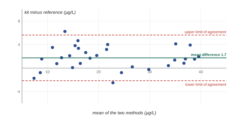
For method comparisons in particular, a test of the mean difference is only part of the story. A Bland–Altman plot, which graphs the difference against the mean of the two measurements for each sample, shows whether the bias is constant or changes with concentration and gives limits of agreement (mean difference ± 1.96 SD of differences) within which most individual differences fall. CHEM-213 discusses method validation in more depth.
Independent samples: the two-sample t test
When the two groups contain different, unrelated units, the comparison is of two independent means. The test statistic divides the difference in sample means by its standard error. There are two versions. The pooled (Student) t test assumes the two populations have equal variances and combines the sample variances into one estimate. Welch’s t test does not assume equal variances; it uses each group’s own variance and an adjusted number of degrees of freedom.
Welch’s test performs almost as well as the pooled test when variances are equal and much better when they are not, especially when the group sizes also differ. Many statisticians therefore recommend Welch’s test as the default for comparing two independent means. In scipy, stats.ttest_ind uses the pooled test unless equal_var=False is given.
import numpy as np
from scipy import stats
rng = np.random.default_rng(1520)

# Invented: shell length (mm) of snails from a sheltered and an exposed shore
sheltered = np.round(rng.normal(24.0, 2.0, 18), 1)
exposed = np.round(rng.normal(21.5, 4.0, 12), 1)

for name, x in [("sheltered", sheltered), ("exposed", exposed)]:
    print(f"{name:9s}: n = {x.size}, mean = {x.mean():.2f}, SD = {x.std(ddof=1):.2f}")

w = stats.ttest_ind(sheltered, exposed, equal_var=False)
p = stats.ttest_ind(sheltered, exposed, equal_var=True)
ci = w.confidence_interval(0.95)
print(f"Welch:  t = {w.statistic:.2f}, df = {w.df:.1f}, p = {w.pvalue:.4f}, "
      f"95% CI {ci.low:.2f} to {ci.high:.2f} mm")
print(f"Pooled: t = {p.statistic:.2f}, df = {p.df:.0f}, p = {p.pvalue:.4f}")sheltered: n = 18, mean = 24.60, SD = 1.98 exposed : n = 12, mean = 21.62, SD = 4.40 Welch: t = 2.20, df = 14.0, p = 0.0453, 95% CI 0.07 to 5.88 mm Pooled: t = 2.52, df = 28, p = 0.0175
The two tests disagree noticeably here. The exposed shore has both the smaller sample and the larger spread, and the pooled test, by averaging the two variances, understates the uncertainty in the exposed-shore mean, so its p-value is too small. Welch’s test gives weaker but more honest evidence of a difference, with an interval that barely excludes zero.
The simulation below shows why Welch’s test is the safer default. When the smaller group has the larger variance and there is no true difference, the pooled test rejects H₀ far more often than the nominal 5 percent.
import numpy as np
from scipy import stats
rng = np.random.default_rng(15109)
reps = 10_000
rej_pooled = rej_welch = 0
for _ in range(reps):
    a = rng.normal(0, 1, 30)     # larger group, smaller SD
    b = rng.normal(0, 3, 10)     # smaller group, larger SD; same mean
    rej_pooled += stats.ttest_ind(a, b).pvalue < 0.05
    rej_welch += stats.ttest_ind(a, b, equal_var=False).pvalue < 0.05
print(f"false positive rate, pooled t: {rej_pooled/reps:.3f}")
print(f"false positive rate, Welch t: {rej_welch/reps:.3f}")false positive rate, pooled t: 0.204 false positive rate, Welch t: 0.051
Checking assumptions
The t procedures assume that observations are independent within and between groups, and that each population is approximately normal. Independence comes from the design, through random sampling or random assignment, and cannot be checked from the data alone; violations, such as pseudoreplication, are the most serious. Normality matters less as samples grow, because of the central limit theorem. A practical guide:
| Sample size per group | What to check | Advice |
|---|---|---|
| Under about 15 | Plot the data: dot plot, box plot or normal Q–Q plot | Use t only if the data look roughly symmetric with no outliers |
| About 15 to 40 | Look for strong skewness and outliers | t is usually fine unless skewness is severe |
| Over about 40 | Check for extreme outliers and dependence | t is robust to non-normality; outliers still matter |
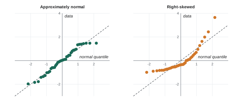
Formal tests of normality, such as the Shapiro–Wilk test, are of limited use: in small samples they lack power to detect important departures, and in large samples they flag trivial ones that do not matter. Graphs are more informative. A normal quantile–quantile (Q–Q) plot compares the ordered data with the values expected from a normal distribution; normal data fall close to a straight line, while curvature indicates skewness and points far from the line at the ends indicate heavy tails or outliers.
When data are right-skewed and positive, as with concentrations, a log transformation often makes them nearly normal, as lesson 4 showed. A t test on log-transformed data compares geometric means, and back-transforming the interval for the difference gives an interval for the ratio of geometric means, which is often the natural scale for concentrations: “the treated soils had 1.6 times the nitrate of the controls (95 percent CI 1.2 to 2.1)”.
Nonparametric alternatives
When data are clearly non-normal, contain outliers, are ordinal (ranked categories such as a pain score from 0 to 10), or come from very small samples, rank-based tests offer an alternative. They replace the data by their ranks and so are not affected by the exact values of extreme observations.
The Wilcoxon signed-rank test is the alternative to the paired t test. It ranks the absolute differences, attaches the signs, and asks whether positive and negative ranks are balanced. The Wilcoxon rank-sum test, also called the Mann–Whitney U test, is the alternative to the two-sample t test. It ranks all observations together and asks whether one group tends to have higher ranks than the other.
import numpy as np
from scipy import stats

# Invented: days to recovery for mice on two treatments, with one extreme value
control = np.array([9, 11, 12, 12, 14, 15, 16, 18, 21, 45])
treated = np.array([6, 7, 8, 9, 9, 10, 11, 12, 13, 15])

t = stats.ttest_ind(control, treated, equal_var=False)
u = stats.mannwhitneyu(control, treated, alternative="two-sided")
print(f"means:   control {control.mean():.1f}, treated {treated.mean():.1f}")
print(f"medians: control {np.median(control):.1f}, treated {np.median(treated):.1f}")
print(f"Welch t test:   p = {t.pvalue:.4f}")
print(f"Mann-Whitney U: U = {u.statistic:.1f}, p = {u.pvalue:.4f}")

# Effect size for Mann-Whitney: probability a control value exceeds a treated value
ps = u.statistic / (control.size * treated.size)
print(f"P(control > treated) estimated as {ps:.2f}")means: control 17.3, treated 10.0 medians: control 14.5, treated 9.5 Welch t test: p = 0.0559 Mann-Whitney U: U = 84.0, p = 0.0110 P(control > treated) estimated as 0.84
The single recovery time of 45 days inflates the control group’s standard deviation, so the Welch test is less convincing, whereas the Mann–Whitney test, which only uses the ranks, gives stronger evidence. The natural effect size for the Mann–Whitney test is the probability of superiority: the chance that a randomly chosen value from one group exceeds one from the other. Here, a control mouse takes longer to recover than a treated mouse about 84 percent of the time.
Nonparametric tests are sometimes described as assumption-free, which is not true. They still require independent observations. The Mann–Whitney test compares whole distributions; it is a test of medians only if the two distributions have the same shape. And when the data really are normal, rank tests are slightly less powerful than t tests, though usually only by about 5 percent. Some researchers prefer to transform data, use bootstrap intervals (lesson 6), or use permutation tests, which shuffle group labels to build the null distribution directly.
import numpy as np
from scipy import stats
rng = np.random.default_rng(1521)
control = np.array([9, 11, 12, 12, 14, 15, 16, 18, 21, 45])
treated = np.array([6, 7, 8, 9, 9, 10, 11, 12, 13, 15])

def diff_medians(x, y, axis=-1):
    return np.median(x, axis=axis) - np.median(y, axis=axis)

res = stats.permutation_test((control, treated), diff_medians, n_resamples=20_000,
                             alternative="two-sided", random_state=rng)
print(f"observed difference in medians = {res.statistic:.1f} days")
print(f"permutation p-value = {res.pvalue:.4f}")observed difference in medians = 5.0 days permutation p-value = 0.0178
Choosing a method
| Design | Data roughly normal or n large | Skewed, ordinal or outliers |
|---|---|---|
| Paired (same or matched units) | Paired t test on differences | Wilcoxon signed-rank test, or t on log ratios |
| Two independent groups | Welch two-sample t test | Mann–Whitney U test, log transform, or permutation test |
| More than two groups | One-way ANOVA (lesson 12) | Kruskal–Wallis test |
Common mistakes
MistakeUse a two-sample t test for before-and-after measurements on the same subjects.
InsteadBefore-and-after data are paired; analyze the differences with a paired t test or signed-rank test.
MistakeAlways use the pooled t test because it has more degrees of freedom.
InsteadUse Welch’s test by default; the pooled test can give too many false positives when variances and sizes differ.
MistakeRun a normality test and switch methods if p < 0.05.
InsteadJudge normality from plots and sample size; formal tests are underpowered for small n and oversensitive for large n.
MistakeNonparametric tests have no assumptions.
InsteadThey still require independence, and the Mann–Whitney test compares medians only when the distributions have the same shape.
MistakeDelete outliers so that the t test works.
InsteadInvestigate outliers; remove them only for documented errors, and otherwise use robust or rank methods and report both analyses.
Summary and key terms
- Paired designs measure the same or matched units twice; analyze the differences.
- Pairing removes between-unit variation and can greatly increase precision.
- For independent groups, Welch’s t test is a safe default because it does not assume equal variances.
- Independence is the most important assumption; normality matters less as n grows.
- Use plots, such as Q–Q plots, rather than formal tests to judge normality.
- Log transformations turn comparisons of skewed concentrations into comparisons of ratios of geometric means.
- The Wilcoxon signed-rank and Mann–Whitney tests are rank-based alternatives; permutation tests build null distributions by shuffling labels.
- paired design
- A design in which observations come in natural pairs, such as before and after measurements on the same unit.
- independent samples
- Samples in which the units in one group are unrelated to those in the other.
- Welch’s t test
- A two-sample t test that does not assume equal population variances.
- pooled variance
- A weighted average of two sample variances used when variances are assumed equal.
- Bland–Altman plot
- A plot of the difference between two methods against their mean, used to assess agreement.
- limits of agreement
- Mean difference ± 1.96 SD of differences between two methods.
- Q–Q plot
- A plot of ordered data against theoretical quantiles, used to check a distributional assumption.
- Wilcoxon signed-rank test
- A rank-based test for paired data.
- Mann–Whitney U test
- A rank-based test comparing two independent groups; also called the Wilcoxon rank-sum test.
- permutation test
- A test that builds the null distribution by repeatedly shuffling group labels.
Practice problems
Work each problem on paper first, then reveal the answer to check.
Blood glucose is measured in 12 patients before and after a diet. Which test is appropriate?
Show answer
A paired t test on the differences, or the Wilcoxon signed-rank test if the differences are skewed.
Ten pairs give mean difference 3.0 and SD of differences 4.0. Compute t.
Show answer
t = 3.0/(4.0/√10) = 2.37, df = 9.
Why does pairing usually increase power?
Show answer
It removes variation between units, so the SD of the differences is smaller than the SD of the raw values.
Group A: n = 20, mean 15.0, SD 3.0. Group B: n = 20, mean 12.0, SD 3.0. Compute the Welch t statistic.
Show answer
SE = √(0.45 + 0.45) = 0.949; t = 3.0/0.949 ≈ 3.16.
When does the pooled t test give misleading results?
Show answer
When variances differ, especially if the smaller group has the larger variance.
What does a curved pattern in a normal Q–Q plot suggest?
Show answer
Skewness; the data are not normal.
A t test on log concentrations gives a 95 percent CI for the difference of 0.10 to 0.45. Interpret it.
Show answer
Back-transform: the ratio of geometric means is between e^0.10 = 1.11 and e^0.45 = 1.57.
Pain is scored 0 to 10 by two independent groups. Which test is suitable?
Show answer
Mann–Whitney U test, because the outcome is ordinal.
Is the Mann–Whitney test always a test of medians?
Show answer
No; only when the two distributions have the same shape.
Describe a permutation test for two groups.
Show answer
Compute the observed statistic, shuffle the group labels many times, recompute the statistic each time, and find the proportion of shuffles at least as extreme as observed.
Lesson quiz · 5 questions
Score 60% or more to complete this lesson.
Create a free account to save your progress, take quizzes and earn a certificate.