
ENGG-401 · Lesson 1 of 12 · 25 min
Engineering economics and cash flow diagrams
Engineers rarely choose between designs on technical merit alone. A pump that uses less energy costs more to buy; a bridge built from weathering steel avoids painting but needs a larger first investment; a data centre cooling plant with free cooling saves electricity for twenty years but must be paid for now. Engineering economics is the discipline of comparing such alternatives in money terms, recognizing that money received or spent at different times does not have the same value. It gives engineers a common language with managers, owners, financiers and the public, and it is part of the professional practice expected of engineers in both Canada and the United States. This first lesson explains what engineering economics is for, where it fits in decision-making, the principles that underlie it, the vocabulary of costs, and the cash flow diagram, the most useful single tool in the subject.
Why engineering economics matters
Every engineering project consumes resources: money, materials, labour and time. Owners want to know whether a project is worth doing, which of several designs gives the best value, how long it will take to pay back, and what could go wrong. Engineers are often the people best placed to estimate the costs and benefits of technical options, so they are expected to analyse them. Engineering economics helps answer questions such as:
- Should a factory replace an old compressor now or keep it running for three more years?
- Is it better to lease or buy a fleet of vehicles?
- Which of three water treatment designs has the lowest life-cycle cost?
- Does an energy retrofit earn more than the company's minimum acceptable rate of return?
- Is a public highway interchange justified by its benefits to road users?
In each case, the analysis turns technical estimates into cash flows over time, applies interest to make them comparable, and produces a measure of worth that supports a decision. The decision itself may also depend on non-monetary factors such as safety, environmental impact, reliability and public acceptance, which the analysis should acknowledge rather than ignore.
The decision-making process
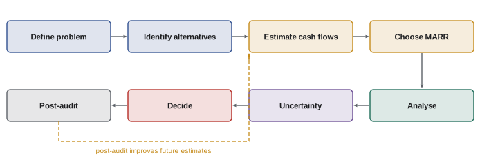
Engineering economic analysis fits within a broader decision process:
- 1. Define the problem and the objective: what need is being met, and what counts as success?
- 2. Identify feasible alternatives, including doing nothing or keeping the existing system, which is often called the do-nothing or base-case alternative.
- 3. Estimate the cash flows of each alternative: first costs, operating and maintenance costs, revenues or savings, salvage values, taxes, and the timing of each.
- 4. Choose the criteria and the interest rate, usually the minimum acceptable rate of return (MARR).
- 5. Analyse the alternatives using present worth, annual worth, rate of return or benefit-cost methods.
- 6. Consider uncertainty through sensitivity, break-even and risk analysis.
- 7. Weigh non-monetary factors and select and implement the preferred alternative.
- 8. Monitor results and compare actual outcomes with estimates, a step called post-audit that improves future estimates.
The quality of the decision depends heavily on step 3: an elegant calculation based on poor estimates produces a misleading answer. Engineers should document their assumptions, state their sources and indicate the uncertainty of their estimates.
Fundamental principles
A few principles underlie all engineering economic analysis:
- Money has a time value. A dollar today is worth more than a dollar next year, because today's dollar can be invested to earn interest, and because people generally prefer to receive money sooner rather than later. Comparing cash flows at different times therefore requires converting them to a common time using an interest rate.
- Only differences between alternatives matter. Costs and revenues that are the same for every alternative do not affect the choice and can be left out, which simplifies analysis.
- Sunk costs are irrelevant. Money already spent cannot be recovered by any future decision, so it should not influence the choice. A company that has spent two million dollars developing a product should decide whether to continue based only on future costs and benefits.
- Marginal revenue must exceed marginal cost. An additional investment is justified only if it earns at least the minimum acceptable return on the extra money spent (Lesson 7).
- Additional risk requires additional return. Riskier projects should be expected to earn more to compensate.
- Cash flows, not accounting profits, determine economic value. Depreciation, for example, is an accounting allocation, not a cash flow, though it affects taxes, which are cash flows (Lesson 9).
The vocabulary of costs
Engineering economists classify costs in several ways:
| Term | Meaning | Example |
|---|---|---|
| First cost (capital cost) | Initial investment to acquire and install an asset | Purchase and installation of a chiller |
| Operating and maintenance (O&M) cost | Recurring costs of running and maintaining | Electricity, labour, spare parts |
| Salvage (residual) value | Net amount recovered at the end of an asset's life | Resale of used equipment minus removal cost |
| Fixed cost | Does not change with output in the relevant range | Rent, insurance, salaried staff |
| Variable cost | Changes in proportion to output | Raw materials, energy per unit produced |
| Sunk cost | Already incurred and unrecoverable | Past research and development spending |
| Opportunity cost | Value of the best alternative forgone | Income lost by using owned land for a project |
| Life-cycle cost | Total cost from conception to disposal | Design, build, operate, maintain, decommission |
Opportunity cost is especially important and often overlooked. If a company uses a building it already owns for a new production line, the building is not free: the company gives up the rent it could have earned by leasing it to someone else, and that rent is a real cost of the project. Similarly, the time of skilled staff assigned to a project has an opportunity cost equal to the value of the work they would otherwise have done.
Cash flows and their conventions
A cash flow is an amount of money received (an inflow, positive) or paid (an outflow, negative) at a particular time. Engineering economics uses a set of conventions to keep analysis consistent:
- Time is divided into periods, usually years, numbered 0, 1, 2 and so on. Time 0 is the present, normally the start of the project.
- Cash flows occurring during a period are assumed to occur at the end of that period, the end-of-period convention. A first cost paid at the start of the project occurs at time 0.
- Net cash flow for a period is inflows minus outflows.
- Standard notation uses \(P\) for a present amount at time 0, \(F\) for a future amount at time \(n\), \(A\) for a uniform series of equal amounts at the end of each period from 1 to \(n\), \(G\) for a uniform gradient (an amount increasing by a constant step each period), \(i\) for the interest rate per period, and \(n\) for the number of periods.
The end-of-period convention is a simplification; real cash flows occur throughout the year. For most decisions, the error is small compared with the uncertainty of the estimates. Where it matters, analyses can use monthly periods or continuous cash flow models (Lesson 2).
Cash flow diagrams
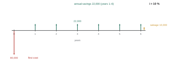
A cash flow diagram is a horizontal time line marked with periods, with arrows representing cash flows: upward arrows for inflows and downward arrows for outflows, drawn roughly to scale. It shows at a glance the size, direction and timing of every cash flow, and it is the best way to set up any engineering economics problem. Drawing a diagram before writing any equations prevents the most common errors, such as misplacing a cash flow by one period, forgetting a salvage value or treating an outflow as an inflow. Diagrams are drawn from one party's point of view: a loan appears as an inflow at time 0 and outflows afterward to the borrower, and the reverse to the lender.
Worked problem
Drawing a cash flow diagram
A manufacturer can buy an automated inspection system for $80,000. It will save $22,000 a year in labour for six years, after which it can be sold for $10,000. Draw the cash flow diagram from the manufacturer's point of view and list the net cash flow in each year.
Show solution
- Draw a time line from 0 to 6.
- Year 0: outflow of $80,000 (downward arrow).
- Years 1 to 5: inflow of $22,000 each (upward arrows).
- Year 6: inflow of $22,000 savings plus $10,000 salvage, a net inflow of $32,000.
Answer: Net cash flows: year 0, −$80,000; years 1–5, +$22,000; year 6, +$32,000.
Estimating cash flows
Estimates come from many sources: vendor quotations, historical cost data, published cost indices, engineering calculations of energy use, labour standards, market studies and expert judgement. Estimates are typically classified by accuracy, from order-of-magnitude estimates used in early screening, often accurate to within −30 % to +50 %, through preliminary and definitive estimates, to detailed estimates based on complete designs and quotations, accurate to within about −5 % to +15 %. Professional organizations such as AACE International publish estimate classification systems used in both countries. Early decisions are often made with the least accurate estimates, which is why sensitivity analysis (Lesson 12) is so important.
Cost indices adjust historical costs to current values. If a similar plant cost $4.2 million when an index stood at 600, and the index now stands at 780, a first estimate of the current cost is:
Capacity changes can be handled with power-sizing, \(C_2 = C_1 (Q_2/Q_1)^x\), where \(x\) is typically between 0.5 and 0.8 for process plants, reflecting economies of scale; the traditional "six-tenths rule" uses \(x = 0.6\).
Professional responsibility
Economic analyses influence large decisions affecting owners, employees and the public. Engineers have a professional duty to make honest, competent estimates, to disclose assumptions and uncertainties, and not to manipulate analyses to favour a preferred outcome. Engineering codes of ethics in both countries require engineers to hold paramount the safety, health and welfare of the public, which means that an alternative cannot be chosen simply because it is cheapest if it compromises safety or violates codes and standards. Economic analysis compares alternatives that are all technically acceptable; it is not a substitute for meeting safety requirements.
In Canada, provincial and territorial regulators such as Professional Engineers Ontario (PEO) and Engineers and Geoscientists BC (EGBC) set codes of ethics that require engineers to act with fairness and loyalty to clients and employers while placing public welfare first, and the Professional Practice Examination (PPE) tests knowledge of these obligations.
Economic analysis across the project life cycle
Economic analysis is not a one-time calculation. In the conceptual phase, rough estimates screen many options and eliminate those that are clearly uneconomic. In the feasibility and preliminary design phases, more detailed estimates compare a short list of alternatives and support the decision to proceed. During detailed design, value engineering studies look for ways to deliver the same function at lower life-cycle cost, for example by changing materials, simplifying details or standardizing components. During construction, change orders and claims are evaluated economically. In operation, decisions about maintenance, upgrades, energy use and replacement continue for decades, and at the end of life, decommissioning and remediation costs must be planned. Engineers who understand this life-cycle perspective make better early decisions, because the greatest opportunity to influence cost occurs early, when designs are still flexible.
Engineering economics and accounting
Engineering economics and accounting use some of the same words with different meanings. Accounting records past transactions and reports profit using rules such as accrual accounting and depreciation schedules; engineering economics looks forward at future cash flows and their timing. A project can show an accounting loss in its early years, because of depreciation and start-up costs, while having a strongly positive present worth; conversely, a project can show accounting profits while destroying value if it earns less than the cost of capital. Engineers should be able to translate between the two views, explaining to accountants and managers why an investment that reduces next year's reported profit is nevertheless worthwhile.
Common mistakes
MistakeIncluding sunk costs in a decision.
InsteadConsider only future cash flows that differ between alternatives.
MistakeForgetting the do-nothing alternative.
InsteadAlways compare against the base case.
MistakeIgnoring opportunity costs of owned assets.
InsteadCharge the value of the best forgone use.
MistakeWriting equations before drawing the cash flow diagram.
InsteadDraw the diagram first to place every cash flow correctly.
MistakePresenting estimates without stating uncertainty.
InsteadDocument assumptions and accuracy ranges.
Summary and key terms
- Engineering economics compares alternatives in money terms over time.
- Decisions follow a process from problem definition to post-audit.
- Money has a time value; only differences between alternatives matter.
- Sunk costs are irrelevant; opportunity costs are real.
- Cash flows are placed at the end of periods using P, F, A, G, i and n.
- Cash flow diagrams show the size, direction and timing of cash flows.
- Estimates vary in accuracy; cost indices and power-sizing adjust historical data.
- Engineering economics
- Analysis of the economic merit of engineering alternatives.
- MARR
- Minimum acceptable rate of return.
- Sunk cost
- Cost already incurred and unrecoverable.
- Opportunity cost
- Value of the best alternative forgone.
- Salvage value
- Net amount recovered at the end of an asset's life.
- Life-cycle cost
- Total cost over an asset's life.
- Cash flow diagram
- Time line showing inflows and outflows.
- End-of-period convention
- Assuming cash flows occur at period ends.
- Cost index
- Ratio used to update historical costs.
- Power-sizing
- Scaling cost with capacity raised to an exponent.
Practice problems
Work each problem on paper first, then reveal the answer to check.
Name four steps in the decision process.
Show answer
Define, identify alternatives, estimate cash flows, choose MARR, analyse, uncertainty, decide, post-audit.
Why are sunk costs irrelevant?
Show answer
No future decision can change them.
Give an example of an opportunity cost.
Show answer
Rent forgone on owned space used for a project.
What does an upward arrow represent?
Show answer
An inflow.
Where is a first cost placed on the diagram?
Show answer
At time 0.
What does A represent?
Show answer
A uniform series of equal end-of-period amounts.
Update a $2 million cost from index 500 to 650.
Show answer
$2.6 million.
Cost of a plant twice the size using x = 0.6?
Show answer
About 1.52 times the original.
Typical accuracy of an order-of-magnitude estimate?
Show answer
About −30 % to +50 %.
Can economics justify an unsafe alternative?
Show answer
No; only technically acceptable alternatives are compared.
Lesson quiz · 5 questions
Score 60% or more to complete this lesson.
Create a free account to save your progress, take quizzes and earn a certificate.