
MATH-100 · Lesson 10 of 12 · 38 min
Areas between curves, RMS values and probability
Lesson 9 introduced the definite integral as an accumulated total and showed how the Fundamental Theorem of Calculus turns its evaluation into antidifferentiation. With that tool in hand, many quantities that would otherwise need laborious summation become single calculations. This lesson develops several applications that appear throughout engineering: reading and using accumulation functions, finding the area between two curves, exploiting symmetry, computing root-mean-square (RMS) values, which determine heating in electrical equipment, and using integrals to describe probabilities, which underlie reliability, quality control and risk. The integrals here require only the antiderivatives you already know; the more advanced techniques of integration, and applications such as volumes and centroids, follow in MATH-101.
Accumulation functions
An accumulation function adds up a rate from a fixed starting point to a variable end:
By the Fundamental Theorem, \(A'(x) = f(x)\): the rate at which the total grows is the value of the integrand at the moving end. This lets you read the behaviour of \(A\) from a graph of \(f\), even when no formula is available. Where \(f > 0\), \(A\) increases; where \(f < 0\), \(A\) decreases; \(A\) has a local maximum where \(f\) changes from positive to negative; and \(A\) is concave up where \(f\) is increasing. All of the curve-sketching ideas of Lesson 6 apply, with \(f\) playing the role of the derivative.
Worked problem
Water in a storage tank
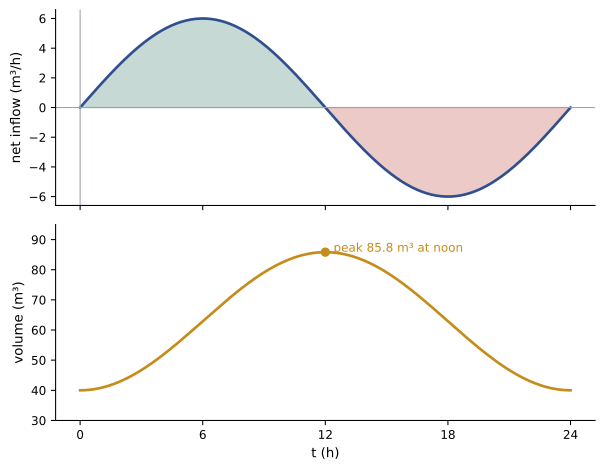
A storage tank holds 40 m³ at midnight. Its net inflow rate (inflow minus outflow) over the next 24 hours is \(r(t) = 6\sin(\pi t / 12)\) m³/h, with \(t\) in hours. When does the tank hold the most water, how much, and how much does it hold at the end of the day?
Show solution
- Volume: \(V(t) = 40 + \int_0^t 6\sin(\pi s/12)\,ds = 40 + \dfrac{72}{\pi}\left(1 - \cos\dfrac{\pi t}{12}\right)\).
- The net inflow is positive for \(0 < t < 12\) and negative for \(12 < t < 24\), so the volume is largest at \(t = 12\): \(V(12) = 40 + \dfrac{144}{\pi} = 85.8\) m³.
- At \(t = 24\): \(V(24) = 40 + \dfrac{72}{\pi}(1 - 1) = 40\) m³.
Answer: The tank peaks at about 85.8 m³ at noon and returns to 40 m³ at midnight. The tank must be sized for the peak, not the starting volume, which is exactly how reservoirs and stormwater ponds are sized from inflow records.
The area between two curves
If \(f(x) \ge g(x)\) on \([a, b]\), the area of the region between their graphs is the integral of the difference, top minus bottom:
Think of slicing the region into thin vertical strips of width \(dx\) and height \(f(x) - g(x)\), and adding them up. If the curves cross, find the intersection points, split the interval there, and integrate the top minus the bottom on each piece. When a region is more naturally bounded by curves written as \(x = h(y)\), slice horizontally instead and integrate right minus left with respect to \(y\).
Worked problem
Area between a parabola and a line
Find the area enclosed by \(y = x^2\) and \(y = 2x + 3\).
Show solution
- Intersections: \(x^2 = 2x + 3\), so \(x^2 - 2x - 3 = (x - 3)(x + 1) = 0\), giving \(x = -1\) and \(x = 3\).
- On \([-1, 3]\), the line is above the parabola (test \(x = 0\): \(3 > 0\)).
- Area: \(\int_{-1}^{3} (2x + 3 - x^2)\,dx = \left[x^2 + 3x - \tfrac{x^3}{3}\right]_{-1}^{3} = (9 + 9 - 9) - (1 - 3 + \tfrac{1}{3}) = 9 + \tfrac{5}{3} = \tfrac{32}{3}\).
Answer: The area is 32/3 ≈ 10.67 square units.
Worked problem
Energy saved by a variable-speed drive
Over an 8-hour shift, a fan with a damper draws \(P_1(t) = 40 - t\) kW, while the same duty with a variable-speed drive draws \(P_2(t) = 22 - 1.5t + 0.1t^2\) kW, with \(t\) in hours. How much energy does the drive save per shift?
Show solution
- Difference: \(P_1 - P_2 = 18 + 0.5t - 0.1t^2\), which is positive on \([0, 8]\) (it equals 15.6 at \(t = 8\)).
- Energy saved: \(\int_0^8 (18 + 0.5t - 0.1t^2)\,dt = \left[18t + 0.25t^2 - \tfrac{0.1t^3}{3}\right]_0^8 = 144 + 16 - 17.07 = 142.9\) kWh.
Answer: About 143 kWh per shift, the area between the two power curves. At $0.12 per kWh and 500 shifts a year, that is about $8,600 a year, the kind of comparison used to justify drives (ELE-470).
Worked problem
Slicing horizontally
Find the area between the curve \(x = y^2\) and the line \(x = 4\).
Show solution
- The region runs from \(y = -2\) to \(y = 2\); for each \(y\), the right boundary is \(x = 4\) and the left is \(x = y^2\).
- Area: \(\int_{-2}^{2} (4 - y^2)\,dy = \left[4y - \tfrac{y^3}{3}\right]_{-2}^{2} = (8 - \tfrac{8}{3}) - (-8 + \tfrac{8}{3}) = \tfrac{32}{3}\).
Answer: 32/3. Slicing vertically would require splitting the region into a top half and a bottom half, so horizontal slices are simpler here.
Using symmetry
Symmetry can halve the work or remove it entirely. If \(f\) is even, \(f(-x) = f(x)\), its graph is symmetric about the \(y\)-axis, and \(\int_{-a}^{a} f(x)\,dx = 2\int_0^a f(x)\,dx\). If \(f\) is odd, \(f(-x) = -f(x)\), the areas on the two sides cancel, and \(\int_{-a}^{a} f(x)\,dx = 0\). For example, \(\int_{-\pi}^{\pi} x^3 \cos x\,dx = 0\) immediately, because \(x^3\cos x\) is odd.
Periodic functions have a similar property: the integral over any complete period is the same, wherever the period starts. In particular, the integral of \(\sin\) or \(\cos\) over a whole number of periods is zero. This fact, combined with the identities for products of sines and cosines, is the foundation of Fourier analysis, which decomposes signals into frequencies (ELE courses).
Root-mean-square values
The average value of a sinusoidal voltage or current over a cycle is zero, yet a resistor connected to an AC supply certainly heats up. The heating depends on the square of the current, since power in a resistor is \(P = i^2 R\). The useful measure is therefore the root-mean-square value: the square root of the average of the square.
A steady direct current equal to \(I_{\text{RMS}}\) produces the same average heating as the varying current. For a sinusoid \(i = I_p \sin\omega t\), the identity \(\sin^2\theta = \tfrac{1}{2}(1 - \cos 2\theta)\) gives an average of \(\sin^2\) over a period of exactly one half, so:
Household voltages are quoted as RMS values: the 120 V supply in North America has a peak of about 170 V, and a 230 V supply a peak of about 325 V.
Worked problem
RMS of a triangular ripple
The ripple current in a converter's capacitor is a symmetric triangle wave that rises linearly from −3 A to +3 A and falls back each period. Find its RMS value.
Show solution
- By symmetry, consider the rising half, where \(i\) goes linearly from −3 to 3 over a time \(T/2\). Let \(u\) run from −1 to 1, so \(i = 3u\).
- Mean of \(i^2\): \(\dfrac{1}{2}\int_{-1}^{1} 9u^2\,du = \dfrac{9}{2} \cdot \dfrac{2}{3} = 3\).
- RMS: \(\sqrt{3} = 1.73\) A, which is the peak divided by \(\sqrt{3}\).
Answer: About 1.73 A. Triangle waves have RMS = peak/√3, sinusoids peak/√2, and square waves RMS = peak. Capacitor and inductor heating calculations (ELE-470) use these results constantly.
Worked problem
A pulsed load
A heater draws 20 A for 3 seconds and nothing for 7 seconds, repeating. Find its average and RMS current, and compare their heating effect in a cable.
Show solution
- Average: \(20 \times 3/10 = 6\) A.
- Mean square: \(20^2 \times 3/10 = 120\) A²; RMS \(= \sqrt{120} = 10.95\) A.
Answer: An average of 6 A but an RMS of about 11 A. The cable heats as if it carried 11 A continuously, so sizing it for 6 A would be unsafe. The more uneven a current, the more its RMS exceeds its average.
Integrals and probability
Many engineering quantities are uncertain: the lifetime of a component, the strength of a batch of concrete, the time between data packets, the error in a measurement. Such a quantity is modelled as a continuous random variable \(X\) with a probability density function \(f(x)\). The density itself is not a probability; instead, the probability that \(X\) falls between \(a\) and \(b\) is the area under the density:
A density must be non-negative and have total area 1, \(\int_{-\infty}^{\infty} f(x)\,dx = 1\), since \(X\) must take some value. The mean, or expected value, is the balance point of the distribution, \(\mu = \int x f(x)\,dx\), a calculation that often needs the integration techniques of MATH-101. STAT-235 develops these ideas fully.
The exponential distribution and reliability
ELE-470, Lesson 2, described components that fail at a constant rate \(\lambda\). Their lifetime \(T\) has the exponential density \(f(t) = \lambda e^{-\lambda t}\) for \(t \ge 0\). The probability of failure by time \(t\) is:
and the probability of surviving beyond \(t\), the reliability, is \(R(t) = e^{-\lambda t}\). The mean lifetime turns out to be \(1/\lambda\), the mean time between failures.
Worked problem
Warranty claims
A power supply fails at a constant rate of \(\lambda = 2 \times 10^{-5}\) per hour of operation. It runs continuously, 8,760 hours a year. What fraction of units fail within a two-year warranty, and what is the probability that a unit survives five years?
Show solution
- Two years: \(\lambda t = 2 \times 10^{-5} \times 17{,}520 = 0.350\); \(P = 1 - e^{-0.350} = 0.295\).
- Five years: \(\lambda t = 0.876\); \(R = e^{-0.876} = 0.416\).
Answer: About 30 percent fail within the warranty and about 42 percent survive five years. A manufacturer facing such numbers would need a more reliable design, which is why the thermal and reliability work in ELE-470 matters commercially.
The uniform and normal distributions
A uniform distribution on \([a, b]\) has constant density \(1/(b - a)\): every value in the interval is equally likely, as with the rounding error of a digital measurement. The normal (Gaussian) distribution, with its bell-shaped density \(f(x) = \frac{1}{\sigma\sqrt{2\pi}} e^{-(x - \mu)^2/(2\sigma^2)}\), describes many measured quantities, but its integral has no elementary antiderivative (Lesson 8), so its probabilities are computed numerically and tabulated. About 68 percent of its area lies within one standard deviation \(\sigma\) of the mean, 95 percent within two, and 99.7 percent within three, figures used throughout quality control.
Worked problem
Rounding error of a meter
A digital thermometer displays whole degrees, so its rounding error is uniformly distributed between −0.5 and +0.5 °C. What is the probability that the error exceeds 0.4 °C in magnitude, and what is the RMS error?
Show solution
- Density: 1 on \([-0.5, 0.5]\). \(P(|E| > 0.4) = 0.1 + 0.1 = 0.2\).
- Mean square: \(\int_{-0.5}^{0.5} e^2\,de = \left[\tfrac{e^3}{3}\right]_{-0.5}^{0.5} = \tfrac{0.25}{3} = 0.0833\); RMS \(= 0.289\) °C.
Answer: A probability of 0.2 and an RMS error of about 0.29 °C, the resolution divided by √12, a standard result in measurement uncertainty.
Common mistakes
MistakeIntegrating f − g without checking which curve is on top.
InsteadFind intersections and integrate top minus bottom on each interval.
MistakeUsing the average current to size a cable for a varying load.
InsteadHeating depends on RMS current.
MistakeTreating a probability density value as a probability.
InsteadProbabilities are areas under the density.
MistakeAssuming a tank is fullest when inflow is highest.
InsteadIt is fullest when the net inflow changes from positive to negative.
MistakeForgetting that odd integrands over symmetric intervals give zero.
InsteadCheck symmetry before integrating.
Summary and key terms
- Accumulation functions grow where the integrand is positive and peak where it changes from positive to negative.
- Area between curves is the integral of top minus bottom, split at intersections; horizontal slices sometimes help.
- Even functions double the half-interval integral; odd functions integrate to zero over symmetric intervals.
- RMS values measure heating: sinusoids peak/√2, triangles peak/√3, square waves peak.
- Probabilities for continuous random variables are areas under a density with total area 1.
- Exponential lifetimes give P(T ≤ t) = 1 − e^(−λt) and mean 1/λ.
- Uniform rounding error has RMS equal to resolution/√12; normal probabilities are tabulated.
- Accumulation function
- A function defined as the integral of a rate from a fixed start to a variable end.
- Area between curves
- The integral of the difference between an upper and a lower function.
- Even function
- A function with f(−x) = f(x).
- Odd function
- A function with f(−x) = −f(x).
- Root-mean-square (RMS)
- The square root of the average of the square of a quantity.
- Probability density function
- A function whose area over an interval gives the probability of that interval.
- Expected value
- The mean of a random variable, ∫x f(x) dx.
- Exponential distribution
- The lifetime distribution for constant failure rate.
- Reliability
- The probability of surviving beyond a given time.
- Uniform distribution
- A distribution with constant density over an interval.
Practice problems
Work each problem on paper first, then reveal the answer to check.
If \(A(x) = \int_0^x (t^2 - 4)\,dt\), where does A have a local minimum for \(x > 0\)?
Show answer
At x = 2, where t² − 4 changes from negative to positive.
Area between \(y = x\) and \(y = x^2\)?
Show answer
∫₀¹ (x − x²) dx = 1/6.
Area between \(y = \sin x\) and \(y = 0\) on \([0, 2\pi]\) (total, not net)?
Show answer
4.
Evaluate \(\int_{-2}^{2} (x^5 - 3x^3 + x)\,dx\).
Show answer
0, since the integrand is odd.
Evaluate \(\int_{-1}^{1} (x^2 + 1)\,dx\) using symmetry.
Show answer
2 × (1/3 + 1) = 8/3.
A sinusoidal current has a peak of 14.1 A. RMS value?
Show answer
About 10 A.
A current is 10 A for 25% of the time and 0 otherwise. Average and RMS?
Show answer
2.5 A and 5 A.
With λ = 10⁻⁴ per hour, probability of failure within 1,000 hours?
Show answer
1 − e^(−0.1) ≈ 0.095.
What is the mean lifetime when λ = 5 × 10⁻⁶ per hour?
Show answer
200,000 hours.
A scale reads to 0.1 g. RMS rounding error?
Show answer
0.1/√12 ≈ 0.029 g.
Lesson quiz · 5 questions
Score 60% or more to complete this lesson.
Create a free account to save your progress, take quizzes and earn a certificate.