Calculus in engineering: modelling and a project

The previous eleven lessons built the tools of single-variable calculus: limits, derivatives and their rules, the shape of graphs, optimization, antiderivatives and differential equations, definite integrals, accumulation, approximation and error. Engineers rarely meet these tools one at a time. A real problem arrives as a question about a physical system, and the engineer must decide which quantities matter, write equations that describe them, choose the right mathematical tools, solve, check and explain the result. This process is called mathematical modelling. This final lesson describes the modelling cycle, works through three case studies that combine several lessons each, offers advice on presenting quantitative results, and sets a course project in which you build and analyse a model of your own.

The modelling cycle

Mathematical modelling follows a cycle that experienced engineers apply almost without thinking:

• Understand the question. What decision does the answer support? What accuracy is needed?
• Identify the variables and parameters, with their units: what changes, what is fixed, and what is unknown.
• State the assumptions. Every model simplifies reality: a tank is a cylinder, drag is proportional to speed, heat loss is steady. Writing the assumptions down makes them easy to question later.
• Formulate the equations, usually from conservation laws (mass, energy, momentum, charge), rate laws and geometry.
• Solve, analytically where possible and numerically where not.
• Check: units, limiting cases (what happens if a parameter is zero or very large?), orders of magnitude, and comparison with data or experience.
• Interpret and communicate the result in terms of the original question, including its uncertainty.
• Refine: if the result is not accurate enough, relax the assumption that matters most and repeat.

The British statistician George Box summarized the attitude this cycle requires: all models are wrong, but some are useful. A model is useful when its simplifications do not affect the decision it supports.

Case study 1: sizing a stormwater storage tank

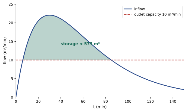
Urban development replaces fields with roofs and pavement, so rain runs off faster and in larger peaks. Municipalities therefore require new developments to store runoff temporarily and release it slowly. Suppose a site's storm inflow to an underground tank is modelled as \(Q_{in}(t) = 2t\,e^{-t/30}\) m³/min, with \(t\) in minutes from the start of the storm, and the outlet releases at most 10 m³/min. How large must the tank be?

• Accumulation (Lessons 9 and 10): storage builds up while inflow exceeds outflow, and is greatest when inflow falls back below outflow. The required volume is the area between the inflow curve and the outflow line, between the times where they cross.
• Finding the crossing times means solving \(2t\,e^{-t/30} = 10\), which has no algebraic solution. Newton's method (Lesson 7) from starting guesses of 6 and 85 minutes gives \(t_1 = 6.13\) min and \(t_2 = 85.0\) min.
• The required antiderivative is not in our table, but it can be found by guessing a form and checking by differentiation: \(\dfrac{d}{dt}\big[-30(t + 30)e^{-t/30}\big] = t\,e^{-t/30}\), which you can verify with the product rule (Lesson 4). MATH-101 shows how to find it systematically by integration by parts.

Case study 2: a falling package with drag

A sensor package is dropped from a drone with a small parachute. Air resistance on the parachute is modelled, as a first approximation, as proportional to speed. How fast does the package fall, how quickly does it reach that speed, and how far does it fall in 10 seconds?

• Newton's second law with gravity and linear drag gives \(\dfrac{dv}{dt} = g - kv\), where \(k\) depends on the parachute and the mass. Measured drop tests give \(k = 1.5\) s⁻¹.
• This is the approach-to-equilibrium equation of Lesson 8, with equilibrium (terminal) velocity \(v_t = g/k\) and time constant \(1/k\).
• Position is the integral of velocity (Lesson 9).

Case study 3: the economic thickness of insulation

Thicker insulation on a heated building costs more to install but saves heating energy every year. The most economical thickness balances the two. For one square metre of wall, suppose the annualized cost of insulation is $0.80 per centimetre of thickness \(x\), and the annual cost of heat lost through the wall is \(\dfrac{63.4}{2 + x}\) dollars, a model derived from the wall's thermal resistance, the local heating degree-days and the price of energy. The total annual cost is:

Presenting quantitative results

A correct calculation is only useful if others can understand and trust it. Good practice includes:

• State the question, the assumptions and the data sources before the results.
• Carry units through every calculation, and check that the units of the answer are right.
• Report a sensible number of significant figures, consistent with the accuracy of the input data: a storage volume computed from a rainfall estimate good to 20 percent should not be reported as 572.64 m³.
• Show the key steps, so that a reviewer can follow and check them, and give limiting-case checks.
• Include a sensitivity analysis: how does the answer change if the most uncertain inputs change? Lesson 5's logarithmic method and Lesson 3's linear approximation make quick sensitivity estimates easy.
• Use graphs to show behaviour, with labelled axes and units.

Professional engineers sign and seal designs that depend on such calculations, and engineering regulators in Canada and the United States hold them responsible for their accuracy. Clear, checkable calculations protect the public and the engineer.

The course project

Choose one of the following problems, or propose your own of similar scope with your instructor's approval, and write a short technical report.

• Project A: Stormwater storage. For a site of your choice, model a storm inflow with a function of the form \(Q(t) = a\,t\,e^{-t/b}\), choose parameters that match a stated peak flow and time to peak, and find the storage required for two outlet capacities. Use Newton's method for the crossing times and check the volume with the trapezoid rule.
• Project B: Cooling or heating. Collect temperature measurements of a cooling object (a mug of hot water, a laptop power adapter after unplugging) at regular intervals. Fit Newton's law of cooling using a semi-logarithmic plot, estimate the time constant, compare the model's predictions with later measurements, and estimate derivatives from your data with central differences.
• Project C: Optimization. Model a design trade-off with a cost or performance function of one variable (insulation thickness, pipe diameter versus pumping energy, the dimensions of a container of fixed volume), find the optimum with calculus, and analyse how it changes with the main parameters.

The report should include:

• A statement of the problem and the decision it supports.
• Variables, parameters with units, and assumptions.
• The model equations, with their origin explained.
• Analytical solutions where possible, and numerical methods (with a convergence check) where not.
• At least one graph, produced by hand or software and checked against your analysis of its shape.
• Checks of units, limiting cases and orders of magnitude.
• A sensitivity analysis of at least two parameters.
• Conclusions and a discussion of the model's limitations and how it could be refined.

Looking ahead

Calculus continues in several directions in the courses that follow. MATH-101 develops techniques of integration, applications such as volumes, work and centroids, and infinite series, including Taylor series. MATH-125 introduces linear algebra, the mathematics of systems of equations and transformations. MATH-209 extends calculus to functions of several variables, and MATH-201 treats differential equations systematically. Physics, circuits, fluid mechanics, heat transfer, structures and control all use these tools from the first week. The habits built in this course, of reasoning about rates and accumulations, checking answers, and approximating with care, are the foundation for all of them.