Nonlinear systems and the phase plane

Lesson 9 solved linear systems completely with eigenvalues and closed with a first look at a nonlinear one, the predator-prey model. Most real systems are nonlinear: a pendulum swinging through a large angle, a structure whose stiffness changes as it deflects, a chemical reactor whose reaction rate rises exponentially with temperature, an electronic oscillator, a population competing for resources. Nonlinear systems rarely have formulas for their solutions, but they show behaviour that linear systems cannot: several stable states, sustained oscillations of a fixed size that do not depend on how the motion started, and sudden changes as a parameter varies. This lesson develops the geometric tools for understanding them in the phase plane: equilibria and linearization, conserved energy, Lyapunov functions, limit cycles and bifurcations, with numerical simulation as the constant companion.

Equilibria and linearization

A two-dimensional autonomous system is written \(x' = f(x, y)\), \(y' = g(x, y)\). Its equilibria are the points where both rates are zero. Near an equilibrium \((x^*, y^*)\), the system behaves approximately like the linear system with the Jacobian matrix:

The eigenvalues of J classify the equilibrium exactly as in Lesson 9: node, saddle, spiral. A key theorem (Hartman-Grobman) guarantees that this classification carries over to the nonlinear system whenever no eigenvalue has a zero real part. The exception is important: if the linearization predicts a centre (purely imaginary eigenvalues), the nonlinear terms decide whether trajectories spiral in, spiral out or stay closed, and further analysis is needed.

A useful aid for sketching is the set of nullclines: the curves where \(x' = 0\) (trajectories cross them vertically) and where \(y' = 0\) (trajectories cross horizontally). Equilibria lie where nullclines of the two kinds intersect.

The pendulum

A pendulum of length L, with angle \(\theta\) from the downward vertical and light damping c, obeys:

For small angles, \(\sin\theta \approx \theta\) and this is the damped oscillator of Lesson 5. For large angles it is nonlinear. As a system, with \(\omega = \theta'\): \(\theta' = \omega\), \(\omega' = -c\omega - (g/L)\sin\theta\).

Energy and the phase portrait

Without damping, multiplying the equation by \(\theta'\) and integrating shows that the energy (per unit of \(mL^2\)) is conserved:

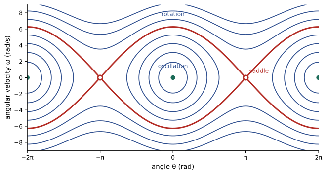
So trajectories are level curves of E, which settles the centre question: near \(\theta = 0\) they are closed loops, and the pendulum swings back and forth forever. At higher energy, the pendulum goes over the top and the trajectory is a wavy line running across the plane: continuous rotation. The boundary between the two, the separatrix, passes through the saddles at \(\theta = \pm\pi\); it is the motion that takes infinitely long to reach the inverted position.

Several stable states: competing species

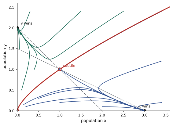
Unlike linear systems, nonlinear systems can have more than one stable equilibrium, and the outcome then depends on where the motion starts. A standard model is two populations competing for the same resource, for example two strains of microorganism in a bioreactor:

Lyapunov functions

Linearization tells us what happens near an equilibrium. A Lyapunov function can prove stability over a larger region, without solving anything. If a function \(V(x, y)\) has a minimum at the equilibrium and never increases along trajectories (\(dV/dt \le 0\)), then the equilibrium is stable; if \(dV/dt < 0\) everywhere except at the equilibrium, every trajectory starting in a region bounded by a level curve of V approaches the equilibrium. Energy is the natural candidate for mechanical and electrical systems.

Limit cycles

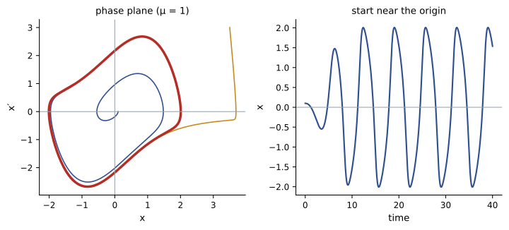
A limit cycle is an isolated closed trajectory: nearby trajectories spiral toward it (a stable limit cycle) or away from it. It represents a self-sustained oscillation of a definite amplitude and frequency, fixed by the system rather than by the initial conditions. Linear systems cannot do this: their closed orbits, as in an undamped oscillator, come in continuous families of every size. The classic example is the Van der Pol oscillator, first studied for vacuum-tube circuits:

The damping term is negative for small \(|x|\), pumping energy in, and positive for large \(|x|\), removing it. Small oscillations grow, large ones shrink, and every trajectory (except the equilibrium itself) approaches a single limit cycle. At the origin the Jacobian is \(\begin{pmatrix} 0 & 1 \\ -1 & \mu \end{pmatrix}\) with eigenvalues of positive real part, an unstable spiral; but trajectories cannot escape to infinity because of the strong damping there. A result for planar systems, the Poincaré-Bendixson theorem, then guarantees a closed orbit in between.

import numpy as np
from scipy.integrate import solve_ivp

def van_der_pol(mu):
    def rhs(t, z):
        x, v = z
        return [v, mu * (1 - x**2) * v - x]
    return rhs

for mu in [0.1, 1.0, 5.0]:
    sol = solve_ivp(van_der_pol(mu), [0, 250], [0.1, 0.0], method="LSODA",
                    rtol=1e-9, atol=1e-9, dense_output=True)
    t = np.linspace(150, 250, 200001)
    x = sol.sol(t)[0]
    ups = t[1:][(x[:-1] < 0) & (x[1:] >= 0)]
    period = np.mean(np.diff(ups))
    print(f"mu = {mu:3.1f}: amplitude {x.max():.3f}, period {period:.2f}")
print(f"Linear oscillator period: {2 * np.pi:.2f}")

mu = 0.1: amplitude 2.000, period 6.29
mu = 1.0: amplitude 2.009, period 6.66
mu = 5.0: amplitude 2.022, period 11.61
Linear oscillator period: 6.28

For small \(\mu\), the cycle is nearly a sine wave of amplitude 2 at the linear frequency. For large \(\mu\), it becomes a relaxation oscillation: slow build-up followed by rapid switching, with a much longer period. Limit cycles are deliberate in electronic oscillators and in the pacemaker cells of the heart; they are unwanted in aircraft wing flutter, brake squeal, galloping power lines and machine-tool chatter, where engineers add damping or change stiffness to eliminate them.

Bifurcations and beyond

As in Lesson 2, equilibria and cycles can appear, disappear or change stability as a parameter varies. In two dimensions a new possibility arises, the Hopf bifurcation: a stable spiral loses stability as its complex eigenvalues cross the imaginary axis, and a limit cycle is born. In the Van der Pol equation this happens as \(\mu\) passes through zero. Flutter of an aircraft wing is a Hopf bifurcation in airspeed: above a critical speed, aerodynamic forces act as negative damping and an oscillation grows until it destroys the structure or settles into a violent limit cycle, so certification requires a margin above the maximum flight speed.

In three or more dimensions, nonlinear systems can be chaotic: deterministic, yet so sensitive to initial conditions that long-term prediction is impossible in practice. Lorenz found this in a simple model of atmospheric convection, and it appears in a periodically driven pendulum and in turbulent flow. The practical lessons are to simulate with tight tolerances, to check results against energy or other invariants, and to judge chaotic systems by their statistics rather than by a single trajectory.