
MATH-201 · Lesson 2 of 12 · 34 min
First-order equations: equilibria, existence and special methods
Lesson 1 solved first-order equations by separation of variables and integrating factors. Many first-order models cannot be solved that way, and even when they can, the formula may hide what an engineer most wants to know: does the system settle down, and to what? Will a small disturbance grow or die away? Is there exactly one solution, so that the model actually predicts something? This lesson takes a more qualitative view. It studies autonomous equations through their equilibria and phase lines, shows how equilibria can appear, disappear or change stability as a parameter changes, states the existence and uniqueness theorem and shows what happens when its conditions fail, and adds two further solution methods, exact equations and the Bernoulli substitution, which handle important nonlinear cases.
Autonomous equations and equilibria
An autonomous equation has a right-hand side that depends only on the unknown, not explicitly on time:
Newton's law of cooling, logistic growth, a tank draining through an orifice and many chemical rate laws are autonomous: the rules do not change with the clock. An equilibrium (or critical point) is a value \(y^*\) with \(f(y^*) = 0\); if the system starts there, it stays there forever. Between equilibria, \(f(y)\) has a constant sign, so solutions move steadily up (where \(f > 0\)) or down (where \(f < 0\)) and can never cross an equilibrium, because uniqueness (below) forbids two solutions from meeting.
All of this can be summarized on a phase line: a vertical line marked with the equilibria and arrows showing the direction of motion between them. An equilibrium is stable (an attractor) if nearby solutions move toward it from both sides, unstable (a repeller) if they move away on both sides, and semi-stable if they approach from one side and leave on the other. For a smooth \(f\), the slope at the equilibrium usually decides: \(f'(y^*) < 0\) means stable, \(f'(y^*) > 0\) unstable.
Worked problem
Logistic growth with harvesting
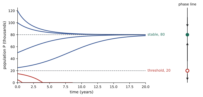
A fish population (in thousands) obeys \(\dfrac{dP}{dt} = 0.5P\left(1 - \dfrac{P}{100}\right) - 8\), the logistic model with a constant harvest of 8 thousand per year. Find the equilibria and their stability.
Show solution
- Set \(0.5P - 0.005P^2 - 8 = 0\), or \(P^2 - 100P + 1600 = 0\), giving \(P = 20\) and \(P = 80\).
- \(f'(P) = 0.5 - 0.01P\): \(f'(20) = 0.3 > 0\) (unstable), \(f'(80) = -0.3 < 0\) (stable).
- Phase line: below 20 the population falls to zero (collapse); between 20 and 80 it rises to 80; above 80 it falls to 80.
Answer: A stable equilibrium at 80 thousand and an unstable threshold at 20 thousand. If the population is ever pushed below 20 thousand, by a bad year or overfishing, it collapses even though the harvest has not changed. Thresholds like this explain the sudden collapse of some fisheries.
Bifurcations
Many models contain a parameter, such as a harvest rate, a feed rate or a supply voltage, and the number or stability of equilibria can change abruptly as it varies. Such a change is a bifurcation. In the harvested logistic model, raising the harvest \(h\) moves the two equilibria toward each other; at \(h = 12.5\) thousand per year they merge at \(P = 50\), and for any larger harvest there is no equilibrium at all: the population declines to zero from any starting value. This saddle-node bifurcation sets the maximum sustainable yield.
Worked problem
Finding the bifurcation point
For \(\dfrac{dP}{dt} = 0.5P\left(1 - \dfrac{P}{100}\right) - h\), find the harvest at which the equilibria merge.
Show solution
- Equilibria satisfy \(0.005P^2 - 0.5P + h = 0\), which has real roots only if the discriminant \(0.25 - 0.02h \ge 0\).
- So \(h \le 12.5\), with the double root \(P = 50\) at \(h = 12.5\).
Answer: h = 12.5 thousand per year, the maximum sustainable harvest. Operating close to it is risky, because the stable equilibrium and the collapse threshold are close together and a small disturbance can push the population over the edge.
Bifurcations appear throughout engineering: a column that stays straight under increasing load until it suddenly buckles (Lesson 6), a chemical reactor that jumps between low- and high-temperature operating states, a power system whose voltage collapses when demand exceeds a critical value, and a fluid flow that changes from steady to oscillating as speed increases.
Existence and uniqueness
A model is useful only if it determines the future: from a given initial state, there should be exactly one solution. The existence and uniqueness theorem guarantees this under mild conditions. For the initial value problem \(y' = f(t, y)\), \(y(t_0) = y_0\): if \(f\) and its partial derivative \(\partial f/\partial y\) are continuous in a region around \((t_0, y_0)\), then there is exactly one solution, at least for some interval of time around \(t_0\).
The conditions are usually satisfied in engineering models, but two kinds of failure are instructive. First, the solution may exist only for a limited time: \(y' = y^2\) with \(y(0) = 1\) has the solution \(y = 1/(1 - t)\), which blows up at \(t = 1\), although the equation looks harmless. Models of runaway processes, such as thermal runaway in batteries, can show this kind of finite-time blow-up. Second, uniqueness can fail where \(\partial f/\partial y\) is infinite.
Worked problem
A leaky bucket
The depth of water in a cylindrical bucket draining through a hole obeys \(h' = -k\sqrt{h}\) (Torricelli). Show that the empty state \(h = 0\) at time \(t = 0\) is consistent with more than one past.
Show solution
- One solution is \(h(t) = 0\) for all \(t\): the bucket was always empty.
- Another is \(h(t) = \tfrac{k^2}{4}(t - T)^2\) for \(t \le T\) and \(h = 0\) after, for any \(T \le 0\): the bucket emptied at time \(T\) and has stayed empty.
- Uniqueness fails because \(\partial f/\partial h = -k/(2\sqrt{h})\) is infinite at \(h = 0\).
Answer: From an empty bucket, you cannot tell when it emptied: the model predicts the future uniquely while water remains, but not the past from an empty state. The square root in Torricelli's law, not any error in the calculation, causes the non-uniqueness.
Exact equations
Some first-order equations come from differentiating a known function along a solution curve. Writing the equation as \(M(x, y)\,dx + N(x, y)\,dy = 0\), it is exact if there is a function \(F(x, y)\) with \(\partial F/\partial x = M\) and \(\partial F/\partial y = N\). Then the equation says \(dF = 0\), and the solutions are the level curves \(F(x, y) = C\). Since mixed partial derivatives are equal (MATH-209), a necessary and (in simple regions) sufficient test for exactness is:
Exact equations arise naturally from conservation laws: if a quantity such as energy is conserved, its level curves are the trajectories of the system.
Worked problem
Solving an exact equation
Solve \((2xy + 3)\,dx + (x^2 + 4y)\,dy = 0\).
Show solution
- Test: \(\partial M/\partial y = 2x\) and \(\partial N/\partial x = 2x\). Exact.
- Integrate \(M\) with respect to \(x\): \(F = x^2y + 3x + g(y)\).
- Match \(\partial F/\partial y = x^2 + g'(y) = x^2 + 4y\), so \(g(y) = 2y^2\).
Answer: The solutions are the curves x²y + 3x + 2y² = C, with C fixed by an initial condition.
Worked problem
Energy in a nonlinear spring
For a mass on a hardening spring, \(m\ddot{x} + kx + \beta x^3 = 0\). Writing \(v = \dot{x}\) and \(\ddot{x} = v\,dv/dx\), show that the motion conserves an energy, and find it.
Show solution
- The equation becomes \(mv\,dv + (kx + \beta x^3)\,dx = 0\), which is exact (and separable).
- Integrating: \(F = \tfrac{1}{2}mv^2 + \tfrac{1}{2}kx^2 + \tfrac{1}{4}\beta x^4 = E\).
Answer: The conserved energy is ½mv² + ½kx² + ¼βx⁴, kinetic plus potential energy. The trajectories in the (x, v) plane are closed curves of constant E, so the mass oscillates forever, a phase-plane picture developed in Lesson 10.
When an equation is not exact, multiplying by a suitable integrating factor can sometimes make it so. The integrating factor of Lesson 1 for linear equations is one example of this idea.
The Bernoulli equation
An equation of the form \(y' + P(t)y = Q(t)y^n\), with \(n \ne 0, 1\), is nonlinear, but the substitution \(u = y^{1-n}\) turns it into a linear equation for \(u\), which the integrating factor method solves. Bernoulli equations describe, among other things, logistic growth, some drag laws and certain chemical kinetics.
Worked problem
Logistic growth by substitution
Solve \(y' = ry - \dfrac{r}{K}y^2\) using the Bernoulli substitution.
Show solution
- Here \(n = 2\), so let \(u = y^{-1}\), \(u' = -y^{-2}y'\). Dividing the equation by \(-y^2\): \(u' + ru = \dfrac{r}{K}\).
- This is linear with integrating factor \(e^{rt}\): \(u = \dfrac{1}{K} + Ce^{-rt}\).
- So \(y = \dfrac{1}{1/K + Ce^{-rt}} = \dfrac{K}{1 + Ae^{-rt}}\) with \(A = KC\).
Answer: The logistic curve, found here without partial fractions. The substitution works because the reciprocal of a logistic population obeys a linear equation.
Scaling to dimensionless form
Before analysing a model, it pays to rescale it so that the variables have no units. In the harvested logistic model, let \(p = P/K\) (population as a fraction of the carrying capacity) and \(\tau = rt\) (time measured in growth times). The equation \(P' = rP(1 - P/K) - h\) becomes \(dp/d\tau = p(1 - p) - H\), with the single dimensionless group \(H = h/(rK)\). Three parameters have collapsed into one, so a single phase line or bifurcation diagram covers every fishery: equilibria exist only for \(H \le 1/4\), which for r = 0.5 per year and K = 100 thousand gives the maximum sustainable harvest of 12.5 thousand per year found above. Dimensionless groups such as this one, and the Reynolds and Biot numbers in fluid mechanics and heat transfer, show which combinations of parameters actually matter and allow results from a laboratory model to be applied to a full-scale system.
Choosing an approach
For a first-order model, an engineer typically asks: Is it separable or linear (Lesson 1)? Is it exact, or a Bernoulli equation? If none of these, is it autonomous, so that a phase line shows its long-term behaviour? If a formula is needed anyway, numerical methods (MATH-300) will provide one. In every case, finding the equilibria and their stability first is cheap and tells you what the solution must do, which is the best check on any formula or simulation.
Common mistakes
MistakeSolving for a formula before checking equilibria.
InsteadFind equilibria and their stability first; they show the long-term behaviour.
MistakeAssuming a solution exists for all time.
InsteadNonlinear equations can blow up in finite time, as y′ = y² does.
MistakeAssuming uniqueness where ∂f/∂y is infinite.
InsteadCheck the conditions of the theorem; square roots often violate them at zero.
MistakeForgetting the function g(y) when building F for an exact equation.
InsteadIntegrate M in x, then find g(y) by matching ∂F/∂y to N.
MistakeOperating a harvested or loaded system close to a bifurcation without margin.
InsteadNear a saddle-node bifurcation, small disturbances can cause collapse.
Summary and key terms
- Autonomous equations y′ = f(y) are analysed through equilibria where f(y) = 0 and a phase line.
- An equilibrium is stable if f′(y*) < 0 and unstable if f′(y*) > 0.
- Bifurcations change the number or stability of equilibria as a parameter varies; harvesting gives a maximum sustainable yield.
- Existence and uniqueness hold when f and ∂f/∂y are continuous; solutions may still blow up in finite time.
- Torricelli draining shows non-uniqueness where ∂f/∂y is infinite.
- Exact equations M dx + N dy = 0 with M_y = N_x have solutions F(x, y) = C, often conserved energies.
- Bernoulli equations become linear with u = y^(1−n).
- Autonomous equation
- A differential equation whose right side does not depend explicitly on time.
- Equilibrium
- A constant solution where the rate of change is zero.
- Phase line
- A diagram of equilibria and directions of motion for an autonomous equation.
- Stable equilibrium
- An equilibrium that nearby solutions approach.
- Bifurcation
- A qualitative change in equilibria as a parameter varies.
- Saddle-node bifurcation
- The merging and disappearance of a stable and an unstable equilibrium.
- Existence and uniqueness theorem
- Conditions guaranteeing exactly one solution of an initial value problem.
- Finite-time blow-up
- A solution becoming infinite at a finite time.
- Exact equation
- An equation M dx + N dy = 0 that is the differential of a function F.
- Bernoulli equation
- y′ + P y = Q yⁿ, made linear by u = y^(1−n).
Practice problems
Work each problem on paper first, then reveal the answer to check.
Find and classify the equilibria of \(y' = y(2 - y)\).
Show answer
y = 0 unstable, y = 2 stable.
Classify the equilibria of \(y' = y^2 - 4\).
Show answer
y = −2 stable, y = 2 unstable.
For \(y' = (y - 1)^2\), what kind of equilibrium is y = 1?
Show answer
Semi-stable: solutions approach from below and leave above.
At what harvest h does \(P' = P(1 - P/40) - h\) lose its equilibria?
Show answer
h = 10.
Does \(y' = 3y^{2/3}\), y(0) = 0, have a unique solution?
Show answer
No; y = 0 and y = t³ both work.
When does the solution of \(y' = y^2\), y(0) = 2, blow up?
Show answer
y = 1/(0.5 − t), at t = 0.5.
Is \((3x^2 + y)\,dx + (x + 2y)\,dy = 0\) exact? Solve it.
Show answer
Yes; x³ + xy + y² = C.
What substitution solves \(y' + y = y^3\)?
Show answer
u = y⁻².
Solve \(y' + y = y^3\) after the substitution.
Show answer
u′ − 2u = −2, u = 1 + Ce^(2t), y = (1 + Ce^(2t))^(−1/2).
Why are exact equations linked to conservation laws?
Show answer
Their solutions are level curves of a conserved function, such as energy.
Lesson quiz · 5 questions
Score 60% or more to complete this lesson.
Create a free account to save your progress, take quizzes and earn a certificate.