Partial derivatives and gradients

In single-variable calculus, the derivative measures how fast a function changes. With several variables, the function can change at different rates in different directions: the temperature in a plate may rise steeply toward a heater and barely change along an insulated edge. Partial derivatives measure the rate of change in each coordinate direction; the gradient packages them into a vector that points uphill and tells you how steep the hill is.

This chapter defines partial derivatives and their meaning, extends linear approximation to several variables (and uses it to estimate measurement errors), develops the multivariable chain rule, introduces directional derivatives and the gradient, and applies them to finding maxima and minima, including constrained optimization with Lagrange multipliers. These ideas are behind heat flow, fluid pressure gradients, error analysis of experiments and every gradient-based optimization algorithm.

Partial derivatives

The partial derivative of \(f(x, y)\) with respect to \(x\) is the ordinary derivative obtained by treating \(y\) as a constant:

Similarly, \(f_y = \partial f/\partial y\) treats \(x\) as a constant. In practice you use all the single-variable rules, holding the other variables fixed.

Geometrically, \(f_x(a, b)\) is the slope of the surface \(z = f(x, y)\) at the point above \((a, b)\), in the x-direction: slice the surface with the plane \(y = b\) and measure the slope of the resulting curve. \(f_y\) is the slope in the y-direction.

Higher derivatives

Partial derivatives can be differentiated again: \(f_{xx}\), \(f_{yy}\), and the mixed partials \(f_{xy} = (f_x)_y\) and \(f_{yx} = (f_y)_x\). For the functions met in engineering (with continuous second partials), Clairaut's theorem guarantees the mixed partials are equal: the order does not matter.

Tangent planes and linear approximation

Close to a point, a smooth surface looks like a plane, just as a smooth curve looks like its tangent line. The tangent plane at \((a, b)\) gives the linear approximation:

The total differential and error propagation

Writing the small changes as differentials gives the total differential:

This is one of the most useful formulas in experimental engineering. If inputs are measured with small uncertainties \(dx\) and \(dy\), the differential estimates the resulting uncertainty in a calculated result. Taking absolute values of each term gives a conservative (worst-case) estimate.

The chain rule

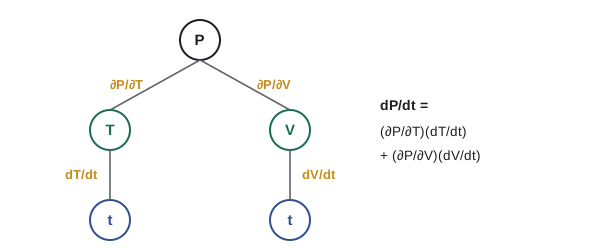
If \(z = f(x, y)\) and both \(x\) and \(y\) change with time, the rate of change of \(z\) collects a contribution from each path:

A tree diagram helps: draw \(z\) at the top, branches to each intermediate variable, branches from those to \(t\), multiply along each path and add the paths.

Directional derivatives and the gradient

Partial derivatives give rates of change along the axes. The rate of change in any direction, given by a unit vector \(\mathbf{u} = (u_1, u_2)\), is the directional derivative:

where the gradient is the vector of partial derivatives:

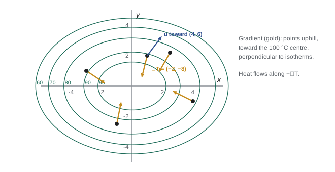
Because \(D_{\mathbf{u}} f = |\nabla f|\cos\theta\), where \(\theta\) is the angle between \(\mathbf{u}\) and the gradient, three facts follow immediately:

• The gradient points in the direction of fastest increase of \(f\), and its magnitude \(|\nabla f|\) is that fastest rate.
• The direction of fastest decrease is \(-\nabla f\).
• The rate of change is zero perpendicular to the gradient, which is the direction along a level curve. So the gradient is always perpendicular to the level curves (and, in 3D, to level surfaces).

The gradient is everywhere in engineering physics. Heat flows down the temperature gradient (Fourier's law, \(\mathbf{q} = -k\nabla T\)); groundwater flows down the hydraulic head gradient (Darcy's law); the electric field is minus the gradient of potential (\(\mathbf{E} = -\nabla V\), PHYS-131); and fluid is pushed by pressure gradients. In each case, the flow crosses the contours at right angles.

Maxima and minima

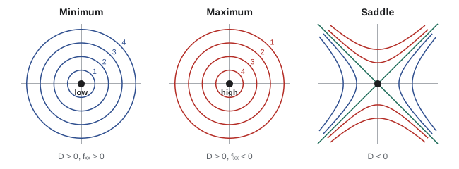
At a smooth local maximum or minimum, the surface is flat: both partial derivatives are zero. Points where \(\nabla f = \mathbf{0}\) (or where a partial derivative does not exist) are critical points. As in one variable, not every critical point is an extreme; in two variables, a critical point can also be a saddle, rising in one direction and falling in another.

The second derivative test sorts them out. At a critical point, compute

• \(D > 0\) and \(f_{xx} > 0\): local minimum.
• \(D > 0\) and \(f_{xx} < 0\): local maximum.
• \(D < 0\): saddle point.
• \(D = 0\): the test is inconclusive.

On a closed, bounded region, a continuous function always has an absolute maximum and minimum. They occur either at critical points inside the region or on its boundary, so check both. This is how you would find, say, the hottest and coldest points of a plate of a given shape.

Optimization with a constraint

Engineering optimization almost always has constraints: minimize material subject to a required volume, maximize strength subject to a weight limit. Sometimes you can substitute the constraint and reduce the number of variables; Lagrange multipliers give a general method. To optimize \(f(x, y, z)\) subject to \(g(x, y, z) = c\), solve

Geometrically, at the optimum the level surface of \(f\) just touches the constraint surface, so their normals (gradients) are parallel.

Gradient-based optimization drives much of modern engineering design software: structural optimization, aerodynamic shape design and the training of machine learning models all repeatedly compute a gradient and step downhill. The ideas in this section are the foundation of those methods.