
MEC-230 · Lesson 4 of 12 · 26 min
Property tables, enthalpy and interpolation
Tomás spent his first week at Northgate shadowing Graham on the morning rounds, writing down pressures and temperatures from gauges all over the plant: boiler outlets, the turbine exhaust, the deaerator, the feedwater pump discharge. Elena then asked him a simple question: how much energy does each kilogram of water carry at each of those points? Answering it means turning two measured properties into the property we actually need, which is usually enthalpy. For water and refrigerants the relations between properties are too complicated for simple equations, so engineers use tables, or software built on the same equations. This lesson is about reading those tables quickly and correctly.
Enthalpy
In the analysis of flowing fluids, internal energy almost always appears together with the product of pressure and specific volume. The combination is so common that it is defined as a property of its own, enthalpy:
Enthalpy is a property because \(u\), \(P\) and \(v\) are properties. Lesson 7 will show where the \(Pv\) term comes from: it is the flow work needed to push each kilogram of fluid into or out of a control volume. For now, note two things. First, in a constant-pressure process in a closed system, the heat transferred equals the change in enthalpy, which is why enthalpy is sometimes loosely called heat content. Second, enthalpy is tabulated alongside internal energy, and for steam it is the property you will use most.
Steam tables list values of \(u\), \(h\) and \(s\) relative to an arbitrary reference state, because thermodynamics deals only with changes in energy. The usual reference sets the internal energy and entropy of saturated liquid water at the triple point (0.01 °C) to zero. Refrigerant tables often use a different reference, so values from different sources can differ by a constant. Changes come out the same whatever the reference, but never mix values from two tables with different references in one calculation.
The saturation tables
Saturated water tables come in two forms: one listed by temperature and one by pressure, so that whichever property is known, the other can be read without interpolation. Each row gives the saturation pressure or temperature and the properties of saturated liquid (subscript \(f\)) and saturated vapour (subscript \(g\)), and often the difference (subscript \(fg\)). The enthalpy of vaporization \(h_{fg}\) is the latent heat introduced in Lesson 3. For mixtures, the quality relations give any property: \(y = y_f + x\,y_{fg}\).
The superheated vapour table
In the superheated region, pressure and temperature are independent, so the table is laid out in blocks, one for each pressure, with rows for a series of temperatures. Each block begins with the saturation temperature at that pressure, in parentheses, and the properties of saturated vapour, followed by rows at higher temperatures. Compared with saturated vapour at the same pressure, superheated vapour has a higher temperature, a larger specific volume, and higher internal energy, enthalpy and entropy.
| T (°C) | v (m³/kg) | h (kJ/kg) | s (kJ/kg·K) |
|---|---|---|---|
| 179.88 (sat.) | 0.19436 | 2777.1 | 6.5850 |
| 200 | 0.20602 | 2828.3 | 6.6955 |
| 250 | 0.23275 | 2943.1 | 6.9265 |
| 300 | 0.25799 | 3051.6 | 7.1246 |
| 350 | 0.28250 | 3158.2 | 7.3029 |
| 400 | 0.30661 | 3264.5 | 7.4670 |
These values describe the steam in the district main. If it leaves the turbine at 1 MPa and 250 °C, it carries 2943.1 kJ/kg; if the turbine is bypassed and the main is fed through a pressure-reducing valve from the 4 MPa header, its temperature after the valve will be higher, as Lesson 8 will show.
Compressed liquid
Compressed-liquid tables exist but are rarely needed, because a liquid's properties depend much more on temperature than on pressure. A common and accurate approximation treats a compressed liquid as a saturated liquid at the same temperature: \(v \approx v_f(T)\), \(u \approx u_f(T)\), \(s \approx s_f(T)\). For enthalpy, which contains the \(Pv\) term, a small correction improves the estimate:
For feedwater at 5 MPa and 80 °C, \(h_f = 335.0\ \text{kJ/kg}\) and the correction adds \(0.001029(5000 - 47.4) = 5.1\ \text{kJ/kg}\), giving 340.1 kJ/kg. The full compressed-liquid table gives about 339 kJ/kg, so the uncorrected value is within about 1 percent and the corrected one within a fraction of a percent. At the very high pressures of supercritical boilers the correction matters more, but at district-energy pressures the simple approximation is usually enough.
Finding the region first
Before reading any table, decide which region the state lies in. Elena's rule for Tomás is to look up the saturation values for whichever property is given, then compare. The flowchart below summarizes the logic for a state given by pressure and one other property.
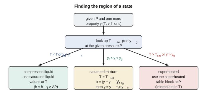
The same logic works with temperature given instead of pressure: compare the pressure with \(P_{\text{sat}}(T)\). If the given pressure is higher, the substance is a compressed liquid (it is squeezed above its boiling pressure); if lower, it is superheated. A frequent slip is to reverse this comparison, so it is worth checking against intuition: water at 1 MPa and 150 °C is below its boiling point of 179.9 °C, so it must be liquid.
Interpolation
Tables cannot list every value, so we interpolate. Over the short intervals in a steam table, properties vary nearly linearly, and linear interpolation is accurate enough for almost all engineering work. For a quantity \(y\) known at \(x_0\) and \(x_1\), its value at \(x\) between them is
Sometimes neither the pressure nor the temperature appears in the table, and we must interpolate twice: first in temperature within each of two pressure blocks, then in pressure between the two results. This double interpolation is tedious by hand, which is why most practising engineers now use property software or a spreadsheet add-in. You should still be able to do it, both for examinations and to check that software output is reasonable.
Worked problem
Enthalpy of steam at an untabulated temperature
Steam in the main is measured at 1 MPa and 280 °C. Find its specific volume, enthalpy and entropy.
Show solution
- The state is superheated, since 280 °C is above \(T_{\text{sat}} = 179.88\ °\text{C}\). Use the 1 MPa block between 250 °C and 300 °C. The interpolation fraction is \((280 - 250)/(300 - 250) = 0.6\).
- \[h = 2943.1 + 0.6(3051.6 - 2943.1) = 2943.1 + 65.1 = 3008.2\ \text{kJ/kg}\]
- Similarly \(v = 0.23275 + 0.6(0.02524) = 0.24789\ \text{m}^3/\text{kg}\) and \(s = 6.9265 + 0.6(0.1981) = 7.0454\ \text{kJ/kg·K}\).
Answer: Each kilogram carries 3008 kJ relative to the triple-point reference. Property software based on the full IAPWS formulation gives a value within about 1 kJ/kg of this, so linear interpolation over a 50 °C interval costs only a few hundredths of a percent here.
Worked problem
Double interpolation
Find the enthalpy of steam at 0.9 MPa and 265 °C, using the 0.8 MPa and 1.0 MPa blocks. At 0.8 MPa: \(h = 2950.4\) at 250 °C and 3057.3 at 300 °C. At 1.0 MPa: 2943.1 and 3051.6.
Show solution
- Interpolate in temperature at each pressure, with fraction \((265 - 250)/50 = 0.3\). At 0.8 MPa: \(h = 2950.4 + 0.3(106.9) = 2982.5\ \text{kJ/kg}\). At 1.0 MPa: \(h = 2943.1 + 0.3(108.5) = 2975.7\ \text{kJ/kg}\).
- Interpolate in pressure, halfway between 0.8 and 1.0 MPa: \(h = (2982.5 + 2975.7)/2 = 2979.1\ \text{kJ/kg}\).
Answer: Enthalpy decreases slightly with pressure at constant temperature in this region, because steam is not an ideal gas; for an ideal gas, as Lesson 5 explains, enthalpy would depend on temperature alone.
The program below automates both interpolations, classifies several states, solves an inverse problem (finding the temperature that gives a known enthalpy, which arises whenever an energy balance gives \(h\) and we need \(T\)), and applies the compressed-liquid correction.
# Locating a state and interpolating in steam tables
# Superheated steam: (P kPa, T C) -> (v m3/kg, h kJ/kg, s kJ/kg.K), rounded from IAPWS-based tables
SUPER = {
    (800, 250): (0.29321, 2950.4, 7.0402),  (800, 300): (0.32416, 3057.3, 7.2348),
    (1000, 250): (0.23275, 2943.1, 6.9265), (1000, 300): (0.25799, 3051.6, 7.1246),
    (1200, 250): (0.19241, 2935.6, 6.8313), (1200, 300): (0.21386, 3046.3, 7.0335),
}
# Saturation: P kPa -> (Tsat C, vf, vg, hf, hg)
SAT = {800: (170.41, 0.001115, 0.24035, 720.9, 2768.3),
       1000: (179.88, 0.001127, 0.19436, 762.5, 2777.1),
       1200: (187.96, 0.001138, 0.16326, 798.3, 2783.8)}

def lerp(x, x0, x1, y0, y1):
    return y0 + (x - x0) / (x1 - x0) * (y1 - y0)

def region(P, T):
    Ts = SAT[P][0]
    if T < Ts - 1e-9: return "compressed liquid"
    if T > Ts + 1e-9: return "superheated"
    return "saturated (need a second property)"

for P, T in ((1000, 150), (1000, 179.88), (1000, 280), (800, 300)):
    print(f"{P:5d} kPa, {T:7.2f} C: {region(P, T)}")

# Single interpolation: 1 MPa, 280 C
v = [lerp(280, 250, 300, a, b) for a, b in zip(SUPER[(1000, 250)], SUPER[(1000, 300)])]
print(f"\n1 MPa, 280 C: v = {v[0]:.5f} m3/kg, h = {v[1]:.1f} kJ/kg, s = {v[2]:.4f} kJ/kg.K")

# Double interpolation: 0.9 MPa, 265 C
def at(P, T):
    return [lerp(T, 250, 300, a, b) for a, b in zip(SUPER[(P, 250)], SUPER[(P, 300)])]
lo, hi = at(800, 265), at(1000, 265)
mid = [lerp(900, 800, 1000, a, b) for a, b in zip(lo, hi)]
print(f"0.9 MPa, 265 C: v = {mid[0]:.5f} m3/kg, h = {mid[1]:.1f} kJ/kg, s = {mid[2]:.4f} kJ/kg.K")

# Inverse problem: 1 MPa steam with h = 3000 kJ/kg -> temperature
h250, h300 = SUPER[(1000, 250)][1], SUPER[(1000, 300)][1]
print(f"1 MPa, h = 3000 kJ/kg: T = {lerp(3000, h250, h300, 250, 300):.1f} C")

# Compressed liquid: feedwater at 5 MPa and 80 C, approximated with saturated liquid at 80 C
Psat80, vf80, hf80 = 47.42, 0.001029, 335.0
print(f"\nfeedwater 5 MPa, 80 C: h ~ hf = {hf80:.1f}; with pressure correction "
f"{hf80 + vf80 * (5000 - Psat80):.1f} kJ/kg")1000 kPa, 150.00 C: compressed liquid 1000 kPa, 179.88 C: saturated (need a second property) 1000 kPa, 280.00 C: superheated 800 kPa, 300.00 C: superheated 1 MPa, 280 C: v = 0.24789 m3/kg, h = 3008.2 kJ/kg, s = 7.0454 kJ/kg.K 0.9 MPa, 265 C: v = 0.27141 m3/kg, h = 2979.1 kJ/kg, s = 7.0423 kJ/kg.K 1 MPa, h = 3000 kJ/kg: T = 276.2 C feedwater 5 MPa, 80 C: h ~ hf = 335.0; with pressure correction 340.1 kJ/kg
Putting it together: Tomás's morning readings
Worked problem
Energy carried at four points in the plant
Tomás's readings, converted to absolute pressure: (a) boiler outlet, 4 MPa and 400 °C; (b) district main, 1 MPa and 280 °C; (c) deaerator outlet, saturated liquid at 120 kPa; (d) condensate returning from a building at 200 kPa and 85 °C. Find the enthalpy at each point. At 4 MPa and 400 °C the table gives \(h = 3214.5\ \text{kJ/kg}\); at 120 kPa, \(h_f = 439.4\); at 85 °C, \(h_f = 356.0\ \text{kJ/kg}\) and \(P_{\text{sat}} = 57.9\ \text{kPa}\).
Show solution
- (a) Superheated, since \(T_{\text{sat}}\) at 4 MPa is 250.4 °C: \(h = 3214.5\ \text{kJ/kg}\) directly from the table.
- (b) Superheated, interpolated in the previous example: \(h = 3008.2\ \text{kJ/kg}\).
- (c) Saturated liquid at 120 kPa (104.8 °C): \(h = h_f = 439.4\ \text{kJ/kg}\).
- (d) 200 kPa is above \(P_{\text{sat}}(85\ °\text{C}) = 57.9\ \text{kPa}\), so the water is compressed liquid. \(h \approx h_f(85\ °\text{C}) = 356.0\ \text{kJ/kg}\); the pressure correction adds only 0.15 kJ/kg.
Answer: Between the condensate return and the boiler outlet, each kilogram of water gains about 2,860 kJ. With a full-load steam flow of 12 kg/s, that is about 34 MW delivered by the boilers, a number we will meet again when we write the first law for control volumes.
Software and the IAPWS formulations
Modern steam tables are generated from equations published by IAPWS. The scientific formulation, IAPWS-95, is a very accurate equation of state for water over the whole fluid range. The industrial formulation, IAPWS-IF97, divides the range into regions with faster equations and is the basis of most commercial software and of contract guarantees for turbines and boilers. Spreadsheet add-ins, online calculators and engineering programs all use one of these. Results from different sources should agree to four or five significant figures; if they do not, suspect a unit or reference-state problem rather than the equations.
Software makes double interpolation obsolete, but it does not remove the need for judgement. It will happily return properties for a state that cannot exist in your system, or interpret 1 MPa as gauge pressure if that is what you typed. The habit of locating the state on a T-v or P-v diagram, and checking that the result is in the right region and of the right size, is what separates a reliable engineer from a fast typist.
Common mistakes
MistakeReading the superheated table for a state that is actually a compressed liquid.
InsteadAlways compare with saturation values first to find the region.
MistakeUsing the saturated-vapour row when the temperature is above T_sat.
InsteadAbove T_sat the state is superheated; use the row at the actual temperature.
MistakeMixing enthalpy values from tables with different reference states.
InsteadChanges are reference-independent, but values from two sources must not be mixed.
MistakeInterpolating in pressure before checking whether each block is in the same region.
InsteadBoth blocks must be in the superheated region at the given temperature.
MistakeUsing the full compressed-liquid correction on internal energy.
Insteadu ≈ u_f(T); the Pv correction applies to enthalpy only.
Summary and key terms
- Enthalpy, h = u + Pv, is a property and the most-used energy quantity for flowing fluids.
- Saturation tables list properties of saturated liquid and vapour by temperature and by pressure.
- Superheated tables are arranged by pressure blocks with rows of temperature.
- A compressed liquid is approximated by saturated liquid at the same temperature, with h ≈ h_f + v_f(P − P_sat).
- Find the region first by comparing a given property with its saturation values.
- Linear interpolation is accurate over table intervals; double interpolation handles untabulated P and T.
- Modern tables and software derive from IAPWS-95 and IAPWS-IF97.
- Enthalpy
- The property h = u + Pv, combining internal energy and flow work.
- Reference state
- The state at which tabulated u and s (or h and s) are set to zero.
- Saturation table
- A table of properties of saturated liquid and vapour, listed by temperature or pressure.
- Superheated vapour table
- A table of properties of vapour above its saturation temperature, arranged by pressure.
- Compressed liquid table
- A table of properties of liquid at pressures above its saturation pressure.
- Linear interpolation
- Estimating a value between two tabulated points by assuming a straight-line variation.
- Double interpolation
- Interpolating in two independent variables, such as pressure and temperature.
- IAPWS-IF97
- The industrial formulation for water and steam properties used in most engineering software.
Practice problems
Work each problem on paper first, then reveal the answer to check.
Steam at 1 MPa and 350 °C: give h and s from the table.
Show answer
h = 3158.2 kJ/kg; s = 7.3029 kJ/kg·K.
Find h for steam at 1 MPa and 225 °C.
Show answer
About 2885.7 kJ/kg.
Water at 4 MPa and 200 °C: which region, and roughly what enthalpy (h_f at 200 °C = 852.2 kJ/kg)?
Show answer
Compressed liquid; h ≈ 852 kJ/kg, or about 855 with the correction.
Steam at 1 MPa has h = 2900 kJ/kg. What is its temperature?
Show answer
About 231 °C, interpolating between 200 °C and 250 °C.
Steam at 1.2 MPa has h = 2700 kJ/kg (h_f = 798.3, h_g = 2783.8). What is its state?
Show answer
A saturated mixture with x = 0.958.
Run the program for 1.1 MPa and 290 °C by adding a second double interpolation. What enthalpy do you get?
Show answer
About 3027 kJ/kg.
Lesson quiz · 5 questions
Score 60% or more to complete this lesson.
Create a free account to save your progress, take quizzes and earn a certificate.