Dirac notation, pictures of quantum dynamics and the time-evolution operator

PHYS-372 used Dirac notation informally, mostly as shorthand for integrals of wave functions. This lesson treats it as what it is: a notation for vectors and linear maps in a Hilbert space that does not depend on any particular basis. With it, the time evolution of a closed system becomes a single object, the unitary time-evolution operator \(U(t, t_0)\). That operator can be attached to the state, to the observables, or partly to each. The three choices are the Schrödinger, Heisenberg and interaction pictures, and the last of them is the starting point for all the perturbation theory in lessons 3 and 4.

Kets, bras and operators

A ket \(|\psi\rangle\) is a vector in a complex Hilbert space \(\mathcal H\). To each ket corresponds a bra \(\langle\psi|\), a linear functional that maps a ket \(|\phi\rangle\) to the complex number \(\langle\psi|\phi\rangle\), the inner product. The inner product is linear in the second slot and antilinear in the first, \(\langle\phi|\psi\rangle = \langle\psi|\phi\rangle^*\), and \(\langle\psi|\psi\rangle \ge 0\) with equality only for the zero vector. The Riesz representation theorem from MATH-445 guarantees that in a Hilbert space every continuous linear functional is a bra of this kind, so the correspondence between kets and bras is one-to-one.

An orthonormal basis \(\{|n\rangle\}\) satisfies \(\langle m|n\rangle = \delta_{mn}\) and the completeness relation

Inserting this identity is the most useful move in the notation. It expands a state as \(|\psi\rangle = \sum_n |n\rangle\langle n|\psi\rangle\), with components \(c_n = \langle n|\psi\rangle\), and it turns an operator into a matrix, \(A = \sum_{mn}|m\rangle\langle m|A|n\rangle\langle n|\), with elements \(A_{mn} = \langle m|A|n\rangle\). The outer product \(|a\rangle\langle b|\) is an operator: acting on \(|\psi\rangle\) it gives \(|a\rangle\langle b|\psi\rangle\). For a continuous basis such as position, sums become integrals and the Kronecker delta becomes a Dirac delta: \(\int dx\,|x\rangle\langle x| = 1\), \(\langle x|x'\rangle = \delta(x - x')\), and the wave function is simply \(\psi(x) = \langle x|\psi\rangle\).

The adjoint \(A^\dagger\) is defined by \(\langle\phi|A^\dagger|\psi\rangle = \langle\psi|A|\phi\rangle^*\); in a basis its matrix is the conjugate transpose. Observables are self-adjoint, \(A = A^\dagger\), and by the spectral theorem have real eigenvalues and a complete set of orthogonal eigenvectors, so \(A = \sum_a a\,P_a\) with \(P_a\) the projection onto the eigenspace for \(a\). A function of an observable is defined through this decomposition, \(f(A) = \sum_a f(a)P_a\). Unitary operators satisfy \(U^\dagger U = UU^\dagger = 1\); they preserve inner products and so map orthonormal bases to orthonormal bases.

The time-evolution operator

For a closed system the Schrödinger equation \(i\hbar\,\partial_t|\psi(t)\rangle = H(t)|\psi(t)\rangle\) is linear, so the state at time \(t\) depends linearly on the state at \(t_0\). Define \(U(t, t_0)\) by \(|\psi(t)\rangle = U(t, t_0)|\psi(t_0)\rangle\). Then

Three properties follow. First, \(U\) is unitary: \(\partial_t(U^\dagger U) = (i/\hbar)U^\dagger(H^\dagger - H)U = 0\) because \(H\) is Hermitian, so \(U^\dagger U\) stays equal to 1 and probabilities are conserved. Second, it has the composition property \(U(t_2, t_0) = U(t_2, t_1)U(t_1, t_0)\): evolving in two stages is the same as evolving at once. Third, \(U(t_0, t) = U(t, t_0)^{-1} = U(t, t_0)^\dagger\), so evolution can be run backward.

If \(H\) does not depend on time, the solution is the operator exponential

where \(|n\rangle\) are the eigenstates of \(H\). The second form is the familiar rule that each stationary state gains a phase \(e^{-iE_nt/\hbar}\). For a time-dependent Hamiltonian that commutes with itself at different times, \([H(t), H(t')] = 0\), the exponent becomes \(-(i/\hbar)\int_{t_0}^tH\,dt'\). In general it does not, and \(U\) must be built from many short steps; lesson 3 expresses the result as a time-ordered exponential.

Numerically, the exponential of a matrix can be computed by the method of scaling and squaring. Divide the matrix by \(2^s\) so that its norm is small, sum the Taylor series \(\sum A^k/k!\) to a modest order, and square the result \(s\) times, using \(e^A = (e^{A/2^s})^{2^s}\). The program uses this method for a spin and for a three-level system and checks unitarity and the composition property directly.

The Schrödinger and Heisenberg pictures

What experiments measure are expectation values and probabilities, such as \(\langle A\rangle_t = \langle\psi(t)|A|\psi(t)\rangle\). Substituting \(|\psi(t)\rangle = U|\psi(0)\rangle\) gives

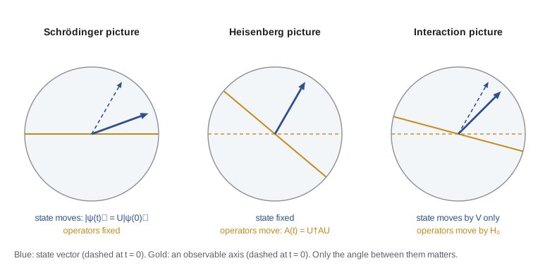
The bracket can be read in two ways. In the Schrödinger picture the state moves, \(|\psi_S(t)\rangle = U|\psi(0)\rangle\), and operators such as \(x\), \(p\) and \(\sigma_z\) are fixed. In the Heisenberg picture the state is fixed at its initial value and the operators move:

The Heisenberg equation of motion, derived by differentiating \(U^\dagger AU\), is the quantum analogue of Hamilton's equations in Poisson-bracket form from PHYS-344, with \(\{A, H\}\) replaced by \([A, H]/i\hbar\). Dirac noticed this correspondence in 1925. For a particle in a potential it gives \(dx_H/dt = p_H/m\) and \(dp_H/dt = -V'(x_H)\), operator equations that look exactly like Newton's laws. Taking expectation values recovers Ehrenfest's theorem.

Heisenberg's own matrix mechanics of 1925 was written in this picture. Schrödinger's wave mechanics of 1926 used the other, and Schrödinger, Dirac and others soon showed that the two give identical predictions, because they differ only by the unitary transformation \(U\). The Heisenberg picture is natural when operators have simple equations of motion, as for the harmonic oscillator, where \(a_H(t) = a\,e^{-i\omega t}\). It is the starting point of quantum field theory, where the operators are fields.

The interaction picture

Suppose \(H = H_0 + V(t)\), where \(H_0\) is simple, such as the Hamiltonian of an atom, and \(V\) is a perturbation, such as the coupling to a light wave. The free evolution \(U_0 = e^{-iH_0t/\hbar}\) is known exactly. The interaction picture removes it from the state and attaches it to the operators:

Differentiating the first definition gives the equation of motion

In this picture the state changes only because of the perturbation. If \(V = 0\) the interaction-picture state is constant. In the eigenbasis of \(H_0\) the matrix elements are \(\langle m|V_I|n\rangle = V_{mn}e^{i\omega_{mn}t}\) with \(\omega_{mn} = (E_m - E_n)/\hbar\), and the components \(c_n = \langle n|\psi_I\rangle\) obey exactly the coupled equations used in PHYS-373 lesson 10. Those equations were the interaction picture in disguise. The picture is named for Dirac, who introduced it in 1927, and it is also called the Dirac picture.

The interaction picture has two advantages. The fast phase oscillations at the Bohr frequencies are removed from the state and appear explicitly as factors \(e^{i\omega_{mn}t}\) in the coupling. And the equation \(i\hbar\,d|\psi_I\rangle/dt = V_I|\psi_I\rangle\) can be solved by iteration, giving the Dyson series of lesson 3, in which each order of perturbation theory is a definite integral.

import cmath, math

def mm(A, B): return [[sum(A[i][k] * B[k][j] for k in range(len(B))) for j in range(len(B[0]))] for i in range(len(A))]
def add(A, B, b=1): return [[A[i][j] + b * B[i][j] for j in range(len(A))] for i in range(len(A))]
def sc(A, c): return [[c * x for x in r] for r in A]
def dag(A): return [[A[j][i].conjugate() for j in range(len(A))] for i in range(len(A))]
def eye(n): return [[1 + 0j if i == j else 0j for j in range(n)] for i in range(n)]
def norm(A): return max(sum(abs(x) for x in r) for r in A)

def expm(A):
    """Matrix exponential by scaling and squaring with a Taylor series."""
    s = max(0, int(math.ceil(math.log2(max(norm(A), 1e-300)))) + 1)
    B = sc(A, 2.0 ** -s); E = eye(len(A)); T = eye(len(A))
    for k in range(1, 20):
        T = sc(mm(T, B), 1 / k); E = add(E, T)
    for _ in range(s): E = mm(E, E)
    return E

def U(H, t): return expm(sc(H, -1j * t))          # hbar = 1
def expect(O, psi): return sum(psi[i].conjugate() * sum(O[i][j] * psi[j] for j in range(len(psi))) for i in range(len(psi))).real
def apply(A, v): return [sum(A[i][j] * v[j] for j in range(len(v))) for i in range(len(A))]

# Spin one-half in a field along z: H = (w/2) sigma_z.  Start along +x.
w = 2 * math.pi           # one full precession per unit time
sx = [[0, 1], [1, 0]]; sy = [[0, -1j], [1j, 0]]; sz = [[1, 0], [0, -1]]
H = sc(sz, w / 2)
psi0 = [1 / math.sqrt(2), 1 / math.sqrt(2)]
print("Spin precession: Schrodinger picture <sx>(t) vs Heisenberg picture")
print("   t     <sx> state evolves   <sx> operator evolves   cos(w t)")
for t in (0.0, 0.125, 0.25, 0.5):
    Ut = U(H, t)
    sch = expect(sx, apply(Ut, psi0))                       # evolve the state
    heis = expect(mm(mm(dag(Ut), sx), Ut), psi0)           # evolve the operator
    print(f"  {t:5.3f}      {sch:+.6f}              {heis:+.6f}             {math.cos(w * t):+.6f}")
print()

# Three-level system (a ladder with couplings): check unitarity and the group property
H3 = [[0, 0.5, 0], [0.5, 1.0, 0.3], [0, 0.3, 2.5]]
U1 = U(H3, 0.7); U2 = U(H3, 1.1); U12 = U(H3, 1.8)
err_unit = norm(add(mm(dag(U1), U1), eye(3), -1))
err_group = norm(add(mm(U2, U1), U12, -1))
print(f"Three-level ladder: ||U^dagger U - 1|| = {err_unit:.1e},  ||U(1.1)U(0.7) - U(1.8)|| = {err_group:.1e}")
psi = apply(U(H3, 3.0), [1, 0, 0])
print("Populations after t = 3.0 starting in level 1:", " ".join(f"{abs(c) ** 2:.4f}" for c in psi), f"(sum {sum(abs(c) ** 2 for c in psi):.12f})")
print()

# Interaction picture: split H = H0 + V; the interaction-picture state changes only because of V
H0 = [[0, 0, 0], [0, 1.0, 0], [0, 0, 2.5]]
V = add(H3, H0, -1)
psiS = apply(U(H3, 3.0), [1, 0, 0])
psiI = apply(dag(U(H0, 3.0)), psiS)                         # |psi_I> = exp(+i H0 t)|psi_S>
print("Interaction-picture amplitudes at t = 3.0:", " ".join(f"{c.real:+.4f}{c.imag:+.4f}i" for c in psiI))
print("Same populations as the Schrodinger picture:", all(abs(abs(a) ** 2 - abs(b) ** 2) < 1e-12 for a, b in zip(psiS, psiI)))

Spin precession: Schrodinger picture <sx>(t) vs Heisenberg picture
   t     <sx> state evolves   <sx> operator evolves   cos(w t)
  0.000      +1.000000              +1.000000             +1.000000
  0.125      +0.707107              +0.707107             +0.707107
  0.250      +0.000000              +0.000000             +0.000000
  0.500      -1.000000              -1.000000             -1.000000

Three-level ladder: ||U^dagger U - 1|| = 6.2e-16,  ||U(1.1)U(0.7) - U(1.8)|| = 3.0e-15
Populations after t = 3.0 starting in level 1: 0.5867 0.3992 0.0141 (sum 1.000000000000)

Interaction-picture amplitudes at t = 3.0: +0.5355+0.5477i +0.6313+0.0250i +0.0747+0.0925i
Same populations as the Schrodinger picture: True

The first table confirms that evolving the state and evolving the operator give the same expectation value, which here is the precession \(\langle\sigma_x\rangle = \cos\omega t\) of a spin in a field along \(z\). The errors in unitarity and composition, near \(10^{-15}\), are rounding errors, showing that scaling and squaring is accurate for small matrices. The interaction-picture amplitudes differ from the Schrödinger ones only by phases, so the populations agree to rounding error, as they must.

Time evolution and conserved quantities

The Heisenberg equation gives an immediate criterion for conservation: an observable \(A\) with no explicit time dependence is conserved exactly when it commutes with \(H\). For a time-independent Hamiltonian, \(H\) itself is conserved. If \([A, H] = 0\), then \(A\) and \(H\) have common eigenstates, and stationary states can be labelled by the eigenvalues of \(A\) as good quantum numbers. Symmetries enter the same way. A symmetry is a unitary operator \(T\) with \(T^\dagger HT = H\), and for continuous symmetries \(T = e^{-i\epsilon G/\hbar}\) the generator \(G\) commutes with \(H\). Translation invariance conserves momentum and rotation invariance conserves angular momentum, the quantum form of Noether's theorem from PHYS-344.

The time-energy relation has a precise form in this language. For a state with energy spread \(\Delta E\) and an observable \(A\), the Mandelstam–Tamm inequality (1945) states that \(\Delta E\,\tau_A \ge \hbar/2\), where \(\tau_A = \Delta A/|d\langle A\rangle/dt|\) is the time for \(\langle A\rangle\) to change by one standard deviation. A state that changes quickly must have a large energy spread. In particular, a quantum gate that turns a state into an orthogonal one in time \(t\) needs \(\Delta E \ge \pi\hbar/2t\), which sets a lower limit on gate times for a given energy scale.