
ROB-340 · Lesson 5 of 12 · 28 min
The SLAM problem
Localization needs a map, and mapping needs to know where the robot is. Simultaneous localization and mapping, SLAM, is the problem of doing both at once, starting with neither. It is often called a chicken-and-egg problem, and for years it was thought to be either impossible or impractically expensive. The breakthrough came from recognizing that the errors in the robot's pose and the errors in its map estimates are correlated, and that keeping track of those correlations makes the problem solvable: when the robot recognizes a place it has seen before, the correction propagates back through the whole map. This lesson defines the SLAM problem precisely, explains why it is hard, and introduces the ideas (online versus full SLAM, data association and loop closure) that the next five lessons build on.
A short history
The probabilistic formulation of SLAM grew out of work in the mid-1980s and early 1990s by Randall Smith, Matthew Self and Peter Cheeseman on representing spatial uncertainty, and by Hugh Durrant-Whyte, John Leonard and colleagues on mobile robot navigation. The acronym SLAM appeared at a robotics symposium in 1995. Through the late 1990s and 2000s, EKF-SLAM, particle-filter methods such as FastSLAM and graph-based methods developed in parallel, and the 2005 textbook Probabilistic Robotics by Sebastian Thrun, Wolfram Burgard and Dieter Fox consolidated the field. Since then, SLAM has moved from laboratories into vacuum cleaners, warehouses, phones (for augmented reality) and cars. A widely cited 2016 survey by Cadena and colleagues asked whether SLAM was solved and answered that it depends on the robot, the environment and the performance required, with robustness and long-term operation the main open problems.
Formulating SLAM
Let \( x_{1:t} \) be the robot's poses up to time t, \( u_{1:t} \) the controls or odometry, \( z_{1:t} \) the measurements and m the map. There are two versions of the problem. Online SLAM estimates only the current pose together with the map:
Full SLAM estimates the entire trajectory together with the map:
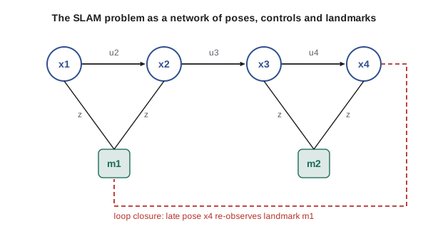
Online SLAM is what a filter computes: at each step it integrates out the past poses. Full SLAM is what a smoother computes: it keeps the past poses, so it can revise them when new information arrives. EKF-SLAM and FastSLAM solve the online problem; graph-based SLAM solves the full problem (or a sliding window of it) and is the dominant approach today, because revisiting past poses fixes linearization errors and handles loop closures cleanly.
The map m can be any of the representations of lesson 2. Feature-based SLAM estimates landmark positions; grid-based SLAM estimates an occupancy grid; pose-graph SLAM estimates only the trajectory and builds the map afterwards from the corrected poses. The structure of the problem is the same: a motion model linking consecutive poses and a measurement model linking poses to the map.
Why SLAM is hard
Four difficulties make SLAM harder than localization or mapping alone. First, the dimension is huge and keeps growing: every new landmark or pose adds variables, so a building-scale map may have hundreds of thousands of unknowns. Second, the pose and map errors are correlated: if the robot's heading is wrong by 2°, every landmark it maps afterwards is rotated by the same 2°, so the errors in the map are not independent of each other or of the pose. Third, data association is uncertain: the robot has to decide which measurements come from which landmarks, or whether the current place is one it has visited before, and a single wrong decision can corrupt the whole map. Fourth, the models are nonlinear: rotations make the motion and measurement models nonlinear, so Gaussian approximations are only valid near the right answer.
The correlations are both the problem and the solution. Because the errors are correlated, re-observing one old landmark accurately tells the robot not only where it is, but also how to correct every other landmark that shares the same accumulated error. Dissanayake and colleagues proved in 2001 that, for linear-Gaussian EKF-SLAM, the landmark uncertainties decrease monotonically and in the limit become fully correlated, so the relative map becomes perfectly known even though its absolute position is limited by the initial uncertainty.
Worked problem
Error growth without loop closure
A robot's odometry drifts at 1.5 % of distance travelled. It drives around a building perimeter of 400 m and returns to its start. How large is the expected position error on return if nothing corrects it? What does that mean for a map built from odometry?
Show solution
- Expected error: \( 0.015 \times 400 = 6 \) m.
- A corridor seen at the start and again at the end would be mapped twice, about 6 m apart.
Answer: About 6 m. The map would show two copies of the start corridor, and every wall in between would be distorted. Recognizing the start (closing the loop) is what lets SLAM remove this error.
Data association
Data association answers the question: which landmark (or which part of the map) does this measurement come from? In feature-based SLAM, it means matching each detected corner, pole or keypoint to an existing landmark or declaring it new. The simplest method is nearest neighbour with a validation gate: compute the Mahalanobis distance between the measurement and each landmark's predicted measurement, using the innovation covariance, and accept the nearest one if the distance falls below a chi-square threshold (ROB-310 lesson 9). Joint compatibility branch and bound (JCBB, Neira and Tardós, 2001) checks that a whole set of associations is mutually consistent, which is much more robust in clutter. Visual SLAM uses descriptor matching plus geometric verification.
Data association errors are the most dangerous failure in SLAM. A filter that incorporates a wrong association becomes confidently wrong, and because it shrinks the covariance, it then rejects the correct measurements that would fix it. Graph-based methods can sometimes detect and remove bad associations afterwards with robust cost functions (lesson 8), which is one reason they have largely replaced filters.
Worked problem
A Mahalanobis validation gate
A range-bearing measurement differs from the predicted measurement of landmark A by innovation \( \nu = (0.30\text{ m}, 0.05\text{ rad}) \). The innovation covariance is diagonal with variances 0.04 m² and 0.0025 rad². Is the association accepted with a 95 % gate for two degrees of freedom (threshold 5.99)?
Show solution
- \( d^2 = 0.30^2/0.04 + 0.05^2/0.0025 = 0.09/0.04 + 0.0025/0.0025 \).
- \( d^2 = 2.25 + 1.00 = 3.25 \).
- 3.25 is below 5.99.
Answer: Yes, the measurement falls inside the 95 % gate and is a plausible match for landmark A. If two landmarks both pass the gate, the association is ambiguous and a joint test or more evidence is needed.
Loop closure
Loop closure is data association on a large scale: recognizing that the robot has returned to a place it has visited before, after travelling far enough that its pose uncertainty is large. Closing a loop lets SLAM remove the drift accumulated around the loop, distributing the correction over all the poses and map elements in between. Without loop closure, SLAM is just odometry with a map attached.
Loop closure has two parts. Place recognition proposes candidate matches, using appearance (bag-of-visual-words methods such as DBoW2 for cameras, scan descriptors such as Scan Context for lidar) or geometry (searching the map near the current uncertain pose). Verification then checks each candidate geometrically, by scan matching or by estimating the relative pose from feature matches with RANSAC, and accepts it only if enough inliers agree. False positives are far worse than false negatives: missing a loop closure leaves some drift, but accepting a wrong one folds two different places together and destroys the map. Systems therefore set conservative thresholds and use robust back ends that can reject closures that conflict with the rest of the graph.
Worked problem
Perceptual aliasing in a warehouse
A warehouse has 30 identical aisles. A place recognizer that ignores geometry proposes a match between the current aisle and a previously visited one. If all aisles look alike and the robot's pose uncertainty spans 5 aisles, what is the chance the proposed match is correct, and what should the system do?
Show solution
- Within the uncertainty region there are 5 equally plausible aisles.
- Without other evidence, the chance any proposed match is correct is about 1 in 5, or 20 %.
- Geometric verification with the robot's odometry prior, or a distinctive landmark at the aisle end, is needed before accepting.
Answer: Only about 20 %. Repetitive environments cause perceptual aliasing; a loop closure there must be verified using geometry and context, or the map can be folded onto the wrong aisle.
Front end and back end
Modern SLAM systems are organized into a front end and a back end. The front end processes raw sensor data: it computes odometry (by scan matching or visual tracking), extracts features, performs data association and proposes loop closures. The back end performs estimation: it takes the constraints produced by the front end and computes the most likely trajectory and map, usually by optimizing a factor graph. This separation means the back end is largely sensor-independent, so the same graph optimizer can serve lidar, camera and multi-sensor systems, while the front end is where most of the sensor-specific engineering, and most of the failures, live.
| Approach | Solves | State representation | Main limitation |
|---|---|---|---|
| EKF-SLAM | Online SLAM | Gaussian over pose and landmarks | Quadratic cost in landmarks; fragile linearization |
| Particle-filter SLAM (FastSLAM, GMapping) | Online (and full per particle) | Particles over trajectories, maps per particle | Particle depletion over long loops |
| Graph-based SLAM | Full or sliding-window SLAM | Factor graph of poses (and landmarks) | Needs good front-end data association |
import numpy as np
rng = np.random.default_rng(4)
# A robot drives a 40 m x 20 m rectangle (120 m) with noisy odometry, 1 m steps
legs = [(40, 0), (20, np.pi / 2), (40, np.pi / 2), (20, np.pi / 2)]
x = y = th = 0.0
for length, turn in legs:
    th += turn + rng.normal(0, np.radians(1.0))         # 1 degree turn error per corner
    for _ in range(length):
        d = 1.0 * (1 + rng.normal(0, 0.01))              # 1 % distance noise
        th += rng.normal(0, np.radians(0.1))             # small heading noise per step
        x += d * np.cos(th); y += d * np.sin(th)
print("odometry end point: (%.2f, %.2f) m; true end point (0, 0)" % (x, y))
print("loop closure error: %.2f m after 120 m (%.1f %% of distance)" % (np.hypot(x, y), 100 * np.hypot(x, y) / 120))odometry end point: (-0.33, -0.23) m; true end point (0, 0) loop closure error: 0.41 m after 120 m (0.3 % of distance)
Common mistakes
MistakeThinking of SLAM as localization followed by mapping
InsteadEstimate pose and map jointly, keeping their correlations.
MistakeAccepting loop closures on appearance alone
InsteadVerify geometrically, and use a robust back end.
MistakeTreating a missed loop closure and a false one as equally bad
InsteadPrefer missing closures; a false closure can destroy the map.
MistakeIgnoring correlations between landmark errors
InsteadTrack them, because re-observing one landmark corrects the others.
MistakeExpecting the absolute map position to become perfectly known
InsteadRelative geometry converges; absolute position is limited by the initial uncertainty unless anchored.
Summary and key terms
- SLAM estimates the robot's pose and the map together, starting with neither.
- Online SLAM estimates the current pose and map; full SLAM estimates the whole trajectory and map.
- SLAM is hard because of high dimension, correlated errors, uncertain data association and nonlinearity.
- Correlated errors are what make SLAM work: re-observing old landmarks corrects the whole map.
- Data association decides which measurements match which landmarks; wrong associations are the most dangerous failure.
- Loop closure recognizes revisited places and removes accumulated drift; false closures are worse than missed ones.
- Modern systems split into a sensor-specific front end and an estimation back end, usually a graph optimizer.
- SLAM
- Simultaneous localization and mapping.
- Online SLAM
- Estimating the current pose and the map.
- Full SLAM
- Estimating the entire trajectory and the map.
- Data association
- Deciding which landmark or map element a measurement comes from.
- Validation gate
- A Mahalanobis-distance threshold for accepting an association.
- JCBB
- Joint compatibility branch and bound, a method that checks sets of associations together.
- Loop closure
- Recognizing a previously visited place and adding the resulting constraint.
- Perceptual aliasing
- Different places that look the same to the sensors.
- Front end
- The part of SLAM that processes sensor data into constraints.
- Back end
- The part of SLAM that estimates the trajectory and map from constraints.
Practice problems
Work each problem on paper first, then reveal the answer to check.
What does online SLAM estimate?
Show answer
The current pose and the map.
What does full SLAM estimate?
Show answer
The whole trajectory and the map.
Name the four main difficulties of SLAM.
Show answer
High dimension, correlated errors, uncertain data association, nonlinearity.
Odometry drift of 2 % over a 250 m loop gives about what error?
Show answer
5 m.
Innovation (0.2 m, 0.1 rad), variances 0.01 m² and 0.01 rad²: what is d²?
Show answer
4 + 1 = 5.
Is d² = 5 inside a 95 % gate for 2 degrees of freedom?
Show answer
Yes, below 5.99.
Why are false loop closures worse than missed ones?
Show answer
They fold different places together and corrupt the map.
Name an appearance-based place recognition method.
Show answer
Bag of visual words, such as DBoW2, or Scan Context for lidar.
What does the SLAM front end do?
Show answer
Processes sensor data into odometry, associations and loop closure constraints.
What does the SLAM back end do?
Show answer
Estimates the trajectory and map from the constraints.
Lesson quiz · 5 questions
Score 60% or more to complete this lesson.
Create a free account to save your progress, take quizzes and earn a certificate.