
ROB-340 · Lesson 8 of 12 · 28 min
Graph-based SLAM
Graph-based SLAM is the approach behind almost every modern SLAM system, from 2-D lidar packages such as slam_toolbox and Cartographer to visual SLAM such as ORB-SLAM and the visual-inertial odometry in phones and headsets. It treats SLAM as an optimization problem: every odometry reading, every landmark observation and every loop closure becomes a constraint between variables, and the best map is the set of variables that satisfies all the constraints as well as possible, in a weighted least-squares sense. Feng Lu and Evangelos Milios proposed the idea in 1997, but it took a decade of work on sparse linear algebra, robust costs and incremental solvers to make it fast and reliable enough for real time. ROB-310 lesson 10 introduced information filters, batch least squares and factor graphs; this lesson applies them to SLAM.
Poses, constraints and the pose graph
A pose graph has one node for each robot pose (in practice, each keyframe or each scan kept for the map) and one edge for each constraint between two poses. An odometry edge links consecutive poses with the relative motion measured by wheel or scan-matching odometry. A loop-closure edge links two poses far apart in time with the relative pose found by matching their scans or images. Each edge carries a measured relative pose \( \mathbf{z}_{ij} \) and an information matrix \( \Omega_{ij} \), the inverse of its covariance, saying how much it should be trusted. Landmarks, if used, become additional nodes with edges to the poses that observed them; a graph with only poses is called a pose graph, and one with both is a full factor graph.
For each edge, define the error as the difference between the measured relative pose and the relative pose predicted from the current node estimates, \( \mathbf{e}_{ij}(x_i, x_j) = \mathbf{z}_{ij} \ominus (x_i^{-1} \oplus x_j) \), where \( \oplus \) and \( \ominus \) compose and differentiate poses with proper angle handling. The SLAM solution minimizes the total weighted squared error:
With Gaussian measurement noise, minimizing F is exactly maximum a posteriori estimation of the full SLAM posterior from lesson 5.
Solving the least-squares problem
F is nonlinear because of rotations, so it is minimized iteratively with Gauss-Newton or Levenberg-Marquardt. At each iteration, every error is linearized around the current estimate, \( \mathbf{e}_{ij}(\mathbf{x} + \Delta\mathbf{x}) \approx \mathbf{e}_{ij} + J_{ij}\Delta\mathbf{x} \), and the minimum of the resulting quadratic is found by solving the normal equations
then updating \( \mathbf{x} \gets \mathbf{x} + \Delta\mathbf{x} \) and repeating until the change is small. Because each edge's Jacobian is non-zero only for its two nodes, H is sparse: its non-zero blocks correspond exactly to edges in the graph. A pose graph with 10,000 nodes has \( 10^8 \) possible blocks in H but only a few tens of thousands of non-zero ones. Sparse Cholesky factorization with a good variable ordering solves such systems in milliseconds, which is why graph SLAM scales where EKF-SLAM could not. One pose must be fixed (or given a strong prior) to remove the gauge freedom: the whole map could otherwise translate and rotate without changing any relative measurement.
Worked problem
A one-dimensional pose graph by hand
A robot moves along a line. Pose \( x_0 = 0 \) is fixed. Odometry says \( x_1 - x_0 = 1.0 \), \( x_2 - x_1 = 1.0 \), \( x_3 - x_2 = 1.0 \), each with variance 0.01. A loop-closure-like measurement says \( x_3 - x_0 = 2.7 \), with variance 0.01. Find the least-squares poses.
Show solution
- The odometry chain predicts \( x_3 = 3.0 \); the direct measurement says 2.7, a conflict of 0.3.
- With equal weights, the 0.3 discrepancy is spread equally over the four constraints in the loop, 0.075 each.
- Each odometry step shrinks to 0.925: \( x_1 = 0.925 \), \( x_2 = 1.850 \), \( x_3 = 2.775 \).
- Check: the direct constraint is now violated by \( 2.775 - 2.7 = 0.075 \), the same as each odometry constraint.
Answer: x1 = 0.925, x2 = 1.85, x3 = 2.775. Least squares shares the conflict among all the constraints in proportion to their uncertainty; a more trusted loop closure would pull harder.
import numpy as np
# Same 1-D graph solved with the normal equations H dx = -b (linear, so one step)
edges = [(0, 1, 1.0), (1, 2, 1.0), (2, 3, 1.0), (0, 3, 2.7)]   # (i, j, measured xj - xi)
info = 1 / 0.01
n = 4
H = np.zeros((n, n)); b = np.zeros(n); x = np.array([0.0, 1.0, 2.0, 3.0])   # odometry guess
for i, j, z in edges:
    e = (x[j] - x[i]) - z
    J = np.zeros(n); J[i], J[j] = -1, 1
    H += info * np.outer(J, J); b += info * J * e
H[0, 0] += 1e6                                   # fix x0 (gauge freedom)
dx = np.linalg.solve(H, -b); x += dx
print("optimized poses:", np.round(x, 3))
print("residuals:", [round(float((x[j] - x[i]) - z), 3) for i, j, z in edges])optimized poses: [0. 0.925 1.85 2.775] residuals: [-0.075, -0.075, -0.075, 0.075]
A two-dimensional pose graph
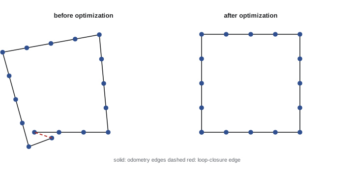
In 2-D each pose is \( (x, y, \theta) \), and the relative pose between nodes i and j, expressed in i's frame, is \( R(\theta_i)^{\mathsf{T}}(\mathbf{t}_j - \mathbf{t}_i) \) for the translation and \( \theta_j - \theta_i \) for the rotation. The error is the difference between this prediction and the measurement, with the angle wrapped into \( (-\pi, \pi] \). The Jacobians follow by differentiation, and each Gauss-Newton step is again a sparse linear solve. The code below builds a square loop of 40 poses with drifting odometry and one loop closure, and optimizes it.
import numpy as np
rng = np.random.default_rng(2)
def wrap(a): return (a + np.pi) % (2 * np.pi) - np.pi
def rel(a, b):                                   # pose of b in a's frame
    c, s = np.cos(a[2]), np.sin(a[2]); d = b[:2] - a[:2]
    return np.array([c * d[0] + s * d[1], -s * d[0] + c * d[1], wrap(b[2] - a[2])])
true = [np.zeros(3)]
for k in range(40):                              # square: 10 x 1 m, then turn 90 deg
    p = true[-1].copy(); turn = np.pi / 2 if k % 10 == 9 else 0
    p[:2] += [np.cos(p[2]), np.sin(p[2])]; p[2] = wrap(p[2] + turn); true.append(p)
edges = []
for k in range(40):                              # noisy odometry edges
    z = rel(true[k], true[k + 1]) + rng.normal(0, [0.02, 0.02, np.radians(1.5)])
    edges.append((k, k + 1, z, np.diag([1 / 0.02**2, 1 / 0.02**2, 1 / np.radians(1.5)**2])))
edges.append((0, 40, rel(true[0], true[40]), np.diag([1e4, 1e4, 1e4])))   # loop closure
x = [np.zeros(3)]
for i, j, z, _ in edges[:-1]:                   # initial guess = integrated odometry
    a = x[-1]; c, s = np.cos(a[2]), np.sin(a[2])
    x.append(np.array([a[0] + c * z[0] - s * z[1], a[1] + s * z[0] + c * z[1], wrap(a[2] + z[2])]))
x = np.array(x)
print("before: end-to-start gap %.2f m" % np.hypot(*(x[40, :2] - x[0, :2])))
for it in range(10):                             # Gauss-Newton
    H = np.zeros((123, 123)); b = np.zeros(123)
    for i, j, z, Om in edges:
        e = rel(x[i], x[j]) - z; e[2] = wrap(e[2])
        c, s = np.cos(x[i, 2]), np.sin(x[i, 2]); d = x[j, :2] - x[i, :2]
        R = np.array([[c, s], [-s, c]]); dR = np.array([[-s, c], [-c, -s]])
        A = np.zeros((3, 3)); A[:2, :2] = -R; A[:2, 2] = dR @ d; A[2, 2] = -1
        B = np.zeros((3, 3)); B[:2, :2] = R; B[2, 2] = 1
        si, sj = slice(3 * i, 3 * i + 3), slice(3 * j, 3 * j + 3)
        H[si, si] += A.T @ Om @ A; H[si, sj] += A.T @ Om @ B
        H[sj, si] += B.T @ Om @ A; H[sj, sj] += B.T @ Om @ B
        b[si] += A.T @ Om @ e; b[sj] += B.T @ Om @ e
    H[:3, :3] += np.eye(3) * 1e9                 # anchor the first pose
    dx = np.linalg.solve(H, -b).reshape(-1, 3); x += dx; x[:, 2] = wrap(x[:, 2])
    if np.abs(dx).max() < 1e-6: break
err = np.mean([np.hypot(*(x[k, :2] - true[k][:2])) for k in range(41)])
print("after %d iterations: gap %.3f m, mean position error %.3f m" % (it + 1, np.hypot(*(x[40, :2] - x[0, :2])), err))before: end-to-start gap 2.38 m after 5 iterations: gap 0.000 m, mean position error 0.184 m
Robust kernels: surviving bad loop closures
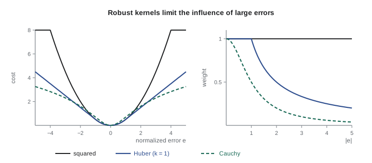
Least squares has a serious weakness: a squared error grows without limit, so a single wrong loop closure with a large error can drag the whole map out of shape to reduce its cost. Since perfect data association cannot be guaranteed, back ends replace the squared cost with a robust kernel \( \rho(e) \) that grows more slowly for large errors. The Huber kernel is quadratic for small errors and linear beyond a threshold; the Cauchy and Geman-McClure kernels flatten out further, so outliers have almost no influence. Robust costs are applied through iteratively reweighted least squares: each iteration down-weights edges with large errors. More specialized methods treat loop closures as switchable constraints (Sünderhauf and Protzel, 2012), dynamic covariance scaling (Agarwal and colleagues, 2013), or graduated non-convexity (Yang and colleagues, 2020), which can reject a large fraction of wrong closures.
Worked problem
Huber weighting of an outlier
A Huber kernel with threshold k = 1 (in units of standard deviations) gives an edge with normalized error |e| the weight \( w = 1 \) if \( |e| \le k \), else \( w = k/|e| \). Two loop closures have normalized errors 0.6 and 12. What weights do they get, and how does that compare with plain least squares?
Show solution
- Edge 1: \( |e| = 0.6 \le 1 \), so w = 1.
- Edge 2: w = 1/12 = 0.083.
- In plain least squares both have weight 1, and edge 2's squared error of 144 dominates the cost.
Answer: The good closure keeps full weight while the suspicious one is down-weighted to about 8 %, so it can no longer distort the map. With a Cauchy or Geman-McClure kernel the outlier's influence would be smaller still.
Incremental and sliding-window solvers
Solving the whole graph from scratch every time a node is added would waste effort, because each new node changes the solution only locally, except at loop closures. Incremental smoothing and mapping, iSAM (Kaess, Ranganathan and Dellaert, 2008) and iSAM2 (2012), keep the factorized system and update it as nodes and edges arrive, re-linearizing only variables whose estimates have changed significantly, using a data structure called the Bayes tree. They give the full-SLAM solution at close to filter cost and are available in the GTSAM library. The other common strategy is a sliding window: optimize only the most recent poses, and marginalize older ones into a prior, which bounds computation; most visual-inertial odometry systems work this way, with a separate global pose graph for loop closures. The g2o and Ceres Solver libraries are also widely used back ends.
| Back end | Approach | Typical use |
|---|---|---|
| g2o | General graph optimization (Gauss-Newton, Levenberg-Marquardt) | Pose graphs, ORB-SLAM, many research systems |
| GTSAM | Factor graphs with iSAM2 incremental solving | Visual-inertial and lidar-inertial SLAM |
| Ceres Solver | General nonlinear least squares | Cartographer, bundle adjustment |
| Karto / slam_toolbox solver | Sparse pose-graph optimization | 2-D lidar SLAM in ROS 2 |
Why graph SLAM won
Compared with filters, graph-based SLAM has three decisive advantages. It re-linearizes, so errors made early in a loop are corrected when better estimates arrive, giving more accurate and more consistent results. It exploits sparsity, so building-scale and city-scale problems are tractable. And it separates the front end from the back end, so loop closures can be added, checked, down-weighted or removed after the fact, which makes systems far more robust to the inevitable association mistakes. Its costs are greater implementation complexity and higher latency at loop closures, when much of the graph may change at once.
Common mistakes
MistakeForgetting to fix one pose or add a prior
InsteadAnchor the graph to remove the gauge freedom, or the system is singular.
MistakeNot wrapping angle errors
InsteadWrap rotational errors into (−π, π] before computing costs.
MistakeGiving loop closures the same tiny covariance regardless of match quality
InsteadSet information matrices from the scan-matching or registration quality.
MistakeUsing plain squared errors with uncertain loop closures
InsteadUse a robust kernel or switchable constraints.
MistakeRe-solving the full dense system every step
InsteadExploit sparsity and use incremental (iSAM2) or sliding-window solvers.
Summary and key terms
- Graph SLAM represents poses (and landmarks) as nodes and measurements as edges with information matrices.
- The best map minimizes the total weighted squared edge error, which is MAP estimation of full SLAM.
- Gauss-Newton linearizes the errors and solves sparse normal equations at each iteration.
- The system is sparse because each edge touches only two nodes, so large graphs solve quickly.
- One pose must be anchored to remove the gauge freedom.
- Robust kernels and switchable constraints limit the damage from wrong loop closures.
- iSAM2 and sliding-window solvers make graph SLAM incremental and real-time.
- Pose graph
- A graph whose nodes are robot poses and whose edges are relative-pose constraints.
- Factor graph
- A graph of variables and the factors (constraints) linking them.
- Information matrix
- The inverse covariance of a constraint, weighting its error.
- Gauss-Newton
- An iterative method that linearizes errors and solves normal equations.
- Normal equations
- The linear system H Δx = −b solved at each Gauss-Newton step.
- Gauge freedom
- The ability of the whole map to move without changing relative measurements.
- Robust kernel
- A cost function that grows slowly for large errors to limit outliers.
- Switchable constraint
- A loop-closure edge with a variable that can turn it off.
- iSAM2
- An incremental smoother that updates the solution as the graph grows.
- Marginalization
- Removing old variables while keeping their information as a prior.
Practice problems
Work each problem on paper first, then reveal the answer to check.
What do the nodes and edges of a pose graph represent?
Show answer
Robot poses, and relative-pose constraints between them.
What does an edge's information matrix express?
Show answer
How much the constraint should be trusted, the inverse covariance.
Why is the normal-equation matrix H sparse?
Show answer
Each edge involves only two nodes.
What must be done to remove gauge freedom?
Show answer
Fix one pose or add a prior.
Three odometry steps of 2.0 each and a direct measurement of 5.7, all equal weight: what is the final pose?
Show answer
5.775 (each constraint absorbs 0.075).
Huber threshold 1, normalized error 4: what weight?
Show answer
0.25.
Name two robust kernels.
Show answer
Huber, Cauchy or Geman-McClure.
What does iSAM2 do?
Show answer
Updates the graph solution incrementally, re-linearizing only where needed.
Name two graph optimization libraries.
Show answer
g2o, GTSAM or Ceres Solver.
Give one advantage of graph SLAM over EKF-SLAM.
Show answer
Re-linearization, sparsity, or the ability to remove bad constraints.
Lesson quiz · 5 questions
Score 60% or more to complete this lesson.
Create a free account to save your progress, take quizzes and earn a certificate.