
ROB-410 · Lesson 2 of 12 · 31 min
Markov decision processes
Reinforcement learning needs a precise way to describe a task: what the robot can observe, what it can do, what happens when it acts and what counts as doing well. The standard framework is the Markov decision process, or MDP. Almost every reinforcement learning algorithm in this course, and many planning and control methods from earlier courses, can be read as a way of solving an MDP. This lesson defines the pieces, introduces returns, discounting and value functions, derives the Bellman equations that tie them together, and discusses what changes when the robot cannot observe the full state.
The agent and the environment
An MDP describes a loop between an agent, here the robot's decision-making system, and an environment, which is everything else: the robot's body, the objects it handles and the physics that connects them. At each discrete time step \( t \), the agent observes the state \( s_t \), chooses an action \( a_t \), receives a scalar reward \( r_{t+1} \) and finds itself in a new state \( s_{t+1} \). The loop then repeats. A sequence of states, actions and rewards from a start state to the end of a task is called an episode or trajectory.
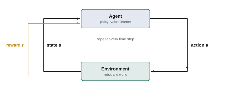
Formally, an MDP is a tuple \( (S, A, P, R, \gamma) \). \( S \) is the set of states and \( A \) the set of actions. \( P(s' \mid s, a) \) is the transition model: the probability of reaching state \( s' \) after taking action \( a \) in state \( s \). \( R(s, a) \) gives the expected reward for taking \( a \) in \( s \). And \( \gamma \in [0, 1] \) is the discount factor, which sets how much the agent values future rewards compared with immediate ones.
The Markov property is the key assumption: the next state and reward depend only on the current state and action, not on the full history. In other words, the state contains everything that matters for predicting the future. For a robot arm, joint angles alone are usually not Markov, because the arm's velocity also affects where it will be next; joint angles and joint velocities together come much closer. Choosing a state representation that is close to Markov is one of the most important modelling decisions in robot learning.
States, actions and rewards for robots
States for robots are usually continuous and high-dimensional. A manipulator's state might include joint positions and velocities, the gripper opening, the pose of the target object and, if the policy works from pixels, one or more camera images. A mobile robot's state might include its pose, velocity and a local map. In practice, the policy rarely sees the true state; it sees observations, such as images and encoder readings, which we return to at the end of the lesson.
Actions can be discrete or continuous. Discrete actions, such as move north, south, east or west in a grid, make the mathematics simple and suit high-level decisions like choosing which object to pick. Low-level robot control almost always uses continuous actions: joint torques, joint velocity targets or Cartesian end-effector displacements. The choice of action space strongly affects learning. Torque actions give the policy full control but make learning harder; position or velocity targets fed to a well-tuned controller from ROB-300 let the policy work at a higher level and usually learn faster.
Rewards encode the task. A sparse reward gives 1 for success and 0 otherwise, which is easy to specify and hard to cheat but gives the learner little signal until it stumbles onto success. A dense or shaped reward adds intermediate terms, such as the negative distance between the gripper and the object, which speed up learning but can introduce unintended behaviour. Lesson 6 is devoted to this trade-off.
Time steps for robots are typically tied to a control rate. A policy might act at 10 Hz to 50 Hz, sending targets to a lower-level controller running at hundreds or thousands of hertz. A 10 s task at 20 Hz is a 200-step episode, which matters when we discuss how discounting spreads credit across time.
| Element | Gridworld example | Robot reaching example |
|---|---|---|
| State | Cell position (row, column) | Joint angles and velocities, target position |
| Action | Up, down, left, right | Joint velocity targets for each joint |
| Transition | Move to neighbouring cell, possibly slipping | Arm dynamics plus controller response |
| Reward | +1 at goal, −1 in a trap, small step cost | Negative distance to target, bonus on arrival |
| Episode end | Goal or trap reached | Target reached or time limit |
Returns and discounting
The agent's goal is not to maximize the next reward but the total reward over time. The return from time \( t \) is the discounted sum of future rewards:
Discounting does three jobs. It keeps the sum finite in tasks that never end. It expresses a preference for getting rewards sooner rather than later. And it controls the effective planning horizon: rewards more than roughly \( 1/(1-\gamma) \) steps away contribute little. With \( \gamma = 0.99 \), the horizon is about 100 steps; with \( \gamma = 0.9 \), about 10 steps. For a 20 Hz controller, \( \gamma = 0.99 \) means the agent effectively looks about 5 s ahead.
The return satisfies a simple recursion that appears again and again: \( G_t = r_{t+1} + \gamma G_{t+1} \). The return now equals the next reward plus the discounted return from the next step.
Worked problem
Computing a discounted return
A robot receives rewards of −1 on each of four steps and then +10 on reaching the goal on step 5, after which the episode ends. Compute \( G_0 \) with \( \gamma = 0.9 \).
Show solution
- The rewards are \( -1, -1, -1, -1, +10 \).
- \( G_0 = -1 - 0.9 - 0.81 - 0.729 + 0.9^4 \times 10 \).
- \( 0.9^4 = 0.6561 \), so the goal term is 6.561.
- Sum of step costs: \( -(1 + 0.9 + 0.81 + 0.729) = -3.439 \).
- \( G_0 = 6.561 - 3.439 = 3.122 \).
Answer: \( G_0 \approx 3.12 \). A longer path to the goal would accumulate more step costs and a smaller discounted bonus, so the agent prefers short paths.
# Discounted returns, computed backwards with G_t = r_{t+1} + gamma * G_{t+1}
import numpy as np
rewards = np.array([-1, -1, -1, -1, 10], dtype=float)
for gamma in (0.9, 0.99, 0.5):
    G = 0.0
    returns = []
    for r in rewards[::-1]:
        G = r + gamma * G
        returns.append(G)
    returns = returns[::-1]
    print(f"gamma={gamma:4}: G_0={returns[0]:7.3f}  all={np.round(returns, 2)}")
for gamma in (0.9, 0.95, 0.99, 0.999):
print(f"gamma={gamma}: effective horizon ~ {1/(1-gamma):.0f} steps")gamma= 0.9: G_0= 3.122 all=[ 3.12 4.58 6.2 8. 10. ] gamma=0.99: G_0= 5.666 all=[ 5.67 6.73 7.81 8.9 10. ] gamma= 0.5: G_0= -1.250 all=[-1.25 -0.5 1. 4. 10. ] gamma=0.9: effective horizon ~ 10 steps gamma=0.95: effective horizon ~ 20 steps gamma=0.99: effective horizon ~ 100 steps gamma=0.999: effective horizon ~ 1000 steps
Policies and value functions
A policy \( \pi \) tells the agent what to do. A deterministic policy maps each state to an action, \( a = \pi(s) \). A stochastic policy gives a probability distribution over actions, \( \pi(a \mid s) \). Stochastic policies are useful for exploration, for representing several equally good ways to act and, as lesson 5 shows, for computing gradients.
The state-value function \( V^\pi(s) \) is the expected return when starting in \( s \) and following \( \pi \) afterwards. The action-value function \( Q^\pi(s, a) \) is the expected return when starting in \( s \), taking action \( a \) first and following \( \pi \) afterwards. Value functions summarize the long-term consequences of being in a state or taking an action, which is exactly the information the agent needs to choose well.
The two are related: \( V^\pi(s) = \sum_a \pi(a \mid s) Q^\pi(s, a) \). The difference \( A^\pi(s, a) = Q^\pi(s, a) - V^\pi(s) \) is called the advantage. It measures how much better action \( a \) is than the policy's average behaviour in that state, and it plays a central role in the policy-gradient methods of lesson 5.
The Bellman equations
Applying the return recursion inside the expectation gives the Bellman expectation equation, which says that the value of a state equals the expected immediate reward plus the discounted value of the next state:
For a finite MDP with \( n \) states, this is a set of \( n \) linear equations in \( n \) unknowns, which can be solved directly: in matrix form \( V = R_\pi + \gamma P_\pi V \), so \( V = (I - \gamma P_\pi)^{-1} R_\pi \). That is policy evaluation in its simplest form.
An optimal policy \( \pi^* \) achieves the highest value in every state. Its value functions, \( V^* \) and \( Q^* \), satisfy the Bellman optimality equations, in which the average over the policy's actions is replaced by a maximum:
Once \( Q^* \) is known, acting optimally is easy: choose \( \pi^*(s) = \arg\max_a Q^*(s, a) \). Much of reinforcement learning is about estimating \( Q^* \) or \( V^* \), either from a known model (lesson 3) or from experience (lesson 4).
# Policy evaluation by solving V = R + gamma P V for a 3-state chain
import numpy as np
# States: 0 = far, 1 = near, 2 = goal (absorbing, zero reward afterwards)
# Policy "advance": from far -> near with prob 0.8 (else stay), near -> goal with 0.9
P = np.array([[0.2, 0.8, 0.0],
              [0.0, 0.1, 0.9],
              [0.0, 0.0, 1.0]])
R = np.array([-1.0, -1.0 + 0.9 * 10, 0.0])   # step cost, plus expected goal bonus from 'near'
gamma = 0.95
V = np.linalg.solve(np.eye(3) - gamma * P, R)
print("V(far), V(near), V(goal) =", np.round(V, 3))
# Check one Bellman equation by hand: V(far) = R(far) + gamma * sum P V
print("check far:", round(R[0] + gamma * P[0] @ V, 3))V(far), V(near), V(goal) = [7.06 8.84 0. ] check far: 7.06
Worked problem
A one-state Bellman check
A robot repeats a task forever. Each cycle it earns reward 2 and stays in the same state. With \( \gamma = 0.9 \), what is \( V \)?
Show solution
- The Bellman equation gives \( V = 2 + 0.9V \).
- So \( 0.1V = 2 \) and \( V = 20 \).
- This matches the geometric series \( 2/(1-0.9) = 20 \).
Answer: \( V = 20 \). The effective horizon of ten steps multiplies the per-step reward by ten.
Episodic, continuing and finite-horizon tasks
Most robot manipulation tasks are episodic: they end when the object is placed, when something goes wrong or when a time limit expires. Time limits need care. If the episode is cut off at 200 steps and the state does not include the time remaining, the cut-off is not part of the Markov state, and value estimates near the limit become confused. Common fixes are to include time remaining in the observation or to treat time-limit endings differently from genuine failures when computing targets, a detail that many practical RL libraries handle explicitly.
Continuing tasks, such as a robot that patrols a warehouse indefinitely, never end and rely on discounting or on average-reward formulations to keep values finite. Finite-horizon formulations, which optimize the sum of rewards over exactly \( H \) steps, connect RL with the model-predictive control that ROB-300 and ROB-350 introduced.
Partial observability
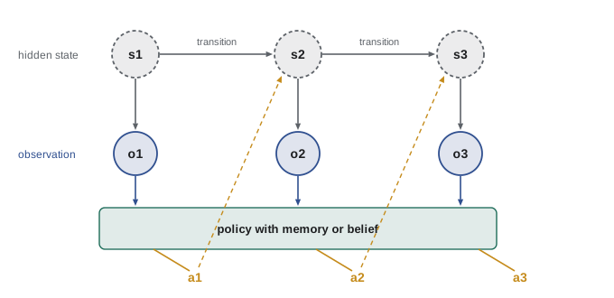
Real robots rarely observe the full state. A camera sees the front of an object but not its mass; a gripper does not know whether an object is about to slip; an occluded object is invisible. The appropriate model is then a partially observable MDP, or POMDP, in which the agent receives observations \( o_t \) drawn from an observation model \( O(o \mid s) \) rather than the state itself.
The theoretically correct approach is to maintain a belief, a probability distribution over states, updated with each observation using the Bayes filter from ROB-310, and to act on that belief. Exact belief planning is intractable for realistic problems, so practical robot learning uses approximations. The most common are stacking the last few observations as input, giving the policy a memory through a recurrent network or a transformer over recent history, or adding explicit state-estimation modules, such as an object-pose tracker, before the policy. Lesson 10 returns to how learned representations help here.
Worked problem
Is this state Markov?
A policy that pushes a puck to a target receives only the puck position from an overhead camera at 10 Hz. Is the observation Markov? What would you add?
Show solution
- The puck may be sliding. Its future position depends on its velocity, which a single position does not reveal.
- The observation is therefore not Markov: two identical positions can lead to different futures.
- Adding the previous position, or an estimated velocity from a filter, restores most of the missing information.
- If friction varies between surfaces, a short history of positions can also let the policy infer how quickly the puck slows down.
Answer: Not Markov. Stack two or more frames, or feed an estimated velocity, so the policy can predict the puck's motion.
Common mistakes
MistakeUsing joint positions alone as the state for a dynamic task.
InsteadInclude velocities, or a short history, so the state is close to Markov.
MistakeSetting \( \gamma \) without thinking about the control rate.
InsteadRelate the effective horizon \( 1/(1-\gamma) \) to the number of steps the task really needs.
MistakeTreating a time-limit cut-off as a failure state.
InsteadInclude time remaining in the observation or bootstrap the value at time-limit endings.
MistakeConfusing \( V \) and \( Q \).
Instead\( V(s) \) values a state under a policy; \( Q(s,a) \) values taking a specific action first.
MistakeAssuming the camera image is the full state.
InsteadRemember partial observability; give the policy memory or explicit state estimates.
Summary and key terms
- An MDP is a tuple of states, actions, transition model, reward function and discount factor.
- The Markov property says the current state contains everything needed to predict the future; choosing such a state is a key design decision.
- The return is the discounted sum of future rewards, and \( 1/(1-\gamma) \) gives the effective horizon in steps.
- Value functions \( V^\pi \) and \( Q^\pi \) give expected returns from states and state-action pairs; the advantage compares an action with the average.
- The Bellman expectation equation is linear and can be solved exactly for small MDPs; the Bellman optimality equation uses a maximum.
- Robot tasks are usually episodic with time limits, which must be handled carefully.
- Real robots face partial observability, handled with observation history, memory or explicit state estimation.
- Markov decision process
- A model of sequential decisions defined by states, actions, transitions, rewards and a discount factor.
- Markov property
- The future depends only on the current state and action, not on earlier history.
- Return
- The discounted sum of future rewards from a given time step.
- Discount factor
- A number between 0 and 1 that weights future rewards relative to immediate ones.
- State-value function
- The expected return from a state when following a given policy.
- Action-value function
- The expected return after taking a given action in a state and then following the policy.
- Advantage
- The difference between an action's value and the state's value under the policy.
- Bellman equation
- A recursive relation expressing a value as immediate reward plus discounted value of successor states.
- POMDP
- A partially observable MDP, in which the agent receives observations rather than the true state.
- Belief
- A probability distribution over possible states given the history of observations and actions.
Practice problems
Work each problem on paper first, then reveal the answer to check.
With \( \gamma = 0.98 \), what is the effective horizon?
Show answer
About \( 1/0.02 = 50 \) steps.
Rewards 0, 0, 5 with \( \gamma = 0.5 \). What is \( G_0 \)?
Show answer
\( 0.5^2 \times 5 = 1.25 \).
Write the recursion linking \( G_t \) and \( G_{t+1} \).
Show answer
\( G_t = r_{t+1} + \gamma G_{t+1} \).
A state earns 1 per step forever with \( \gamma = 0.95 \). What is \( V \)?
Show answer
\( 1/0.05 = 20 \).
Why is a single camera frame often not Markov for a moving object?
Show answer
It shows position but not velocity.
How do you get \( V^\pi \) from \( Q^\pi \)?
Show answer
Average \( Q^\pi(s,a) \) over the policy's action probabilities.
What does a positive advantage mean?
Show answer
The action is better than the policy's average action in that state.
Give one way to handle partial observability.
Show answer
Stack recent observations, use a recurrent or transformer policy, or add a state estimator.
Why might velocity targets be a better action space than torques?
Show answer
A tuned low-level controller handles dynamics, so the policy learns at a higher level and faster.
What is the main drawback of a sparse reward?
Show answer
The learner gets almost no signal until it happens to succeed.
Lesson quiz · 5 questions
Score 60% or more to complete this lesson.
Create a free account to save your progress, take quizzes and earn a certificate.