
ROB-410 · Lesson 9 of 12 · 30 min
Imitation learning II: inverse reinforcement learning and generative policies
Lesson 8 treated demonstrations as input-output pairs to regress. That view leaves two problems unsolved. First, cloning copies actions without understanding why they were taken, so it cannot generalize when the situation changes in ways the data did not cover. Second, real demonstrations are multimodal: the same scene can be handled in several equally good ways, and regression averages them into an action nobody would take. This lesson presents two families of answers. Inverse reinforcement learning recovers the goal behind the demonstrations as a reward function. Generative policies, such as Diffusion Policy and the Action Chunking Transformer, model the full distribution of demonstrated actions. The lesson closes with how demonstration data is collected, since data quality limits everything else.
Inverse reinforcement learning
Reinforcement learning takes a reward and produces behaviour. Inverse reinforcement learning, or IRL, runs the other way: given expert behaviour, find a reward function under which that behaviour is optimal. The motivation is that a reward is a compact, transferable description of a task. A policy that grasps a mug in one kitchen may not work in another, but a reward that says 'mug lifted upright from the counter' applies everywhere, and the robot can re-optimize it in the new setting.
IRL is fundamentally ambiguous. Many rewards explain the same behaviour, including the trivial reward that is zero everywhere, under which every behaviour is optimal. Practical methods add assumptions to pick one. Maximum-margin methods choose the reward under which the expert beats all other policies by the widest margin. Maximum-entropy IRL, introduced by Ziebart and colleagues in 2008, models the expert as choosing trajectories with probability proportional to the exponential of their return, and picks the reward that makes the demonstrations most likely under that model.
Here \( \phi \) is a vector of features, \( \psi \) their weights and \( Z \) a normalizing constant summing over all trajectories. Maximizing the likelihood of demonstrations gives a strikingly simple gradient: the difference between the expert's average feature counts and the feature counts expected under the current reward's soft-optimal policy. Learning stops when the model's behaviour matches the expert's feature statistics.
Worked problem
Feature matching in a reward
A driving reward uses two features per step: speed in metres per second and a penalty feature equal to 1 when within 1 m of another car. Expert demonstrations average 12.0 for speed and 0.02 for proximity per step. The current reward's soft-optimal policy averages 14.5 and 0.10. In which direction should each weight move?
Show solution
- Gradient for speed: \( 12.0 - 14.5 = -2.5 \); the speed weight should decrease, making high speed less attractive.
- Gradient for proximity: \( 0.02 - 0.10 = -0.08 \); the proximity weight should decrease, becoming more negative, so closeness is penalized more.
- Both changes push the model towards the expert's slower, more spacious driving.
Answer: Decrease both weights: less reward for speed and a stronger penalty for proximity.
Classic IRL needs to solve an RL problem inside every iteration, which is expensive. Adversarial imitation methods remove that inner loop. Generative adversarial imitation learning, GAIL, trains a discriminator to tell expert state-action pairs from the policy's, and uses the discriminator's output as the reward for an RL algorithm such as PPO. The policy improves until the discriminator can no longer tell them apart. These methods are powerful in simulation, where RL interaction is cheap, and are used for motion imitation in character animation and legged robots, but they inherit RL's sample cost and are less common for real-world manipulation at the time of writing.
| Approach | Learns | Needs environment interaction? | Typical use |
|---|---|---|---|
| Behaviour cloning | Policy directly | No | Manipulation from teleoperation |
| DAgger | Policy, with expert corrections | Yes, with expert in the loop | Distilling teachers, correcting drift |
| Maximum-entropy IRL | Reward, then policy | Yes, RL inside each iteration | Navigation, driving preferences |
| GAIL and adversarial variants | Policy with learned reward signal | Yes, many RL steps | Motion imitation in simulation |
| Generative policies | Action distribution directly | No | Dexterous, multimodal manipulation |
The multimodality problem
Suppose demonstrators move a gripper around an obstacle, half the time passing to the left and half to the right. A regression policy trained with mean squared error predicts the average action, which aims straight at the obstacle. The same failure appears whenever there are several good choices: which object to pick first, which hand to use, whether to push or lift. Mean squared error assumes a single Gaussian mode, and the average of good actions is often a bad action.
# Multimodal demonstrations: regression averages the modes, a mixture does not
import numpy as np
rng = np.random.default_rng(9)
n = 400
side = rng.choice([-1.0, 1.0], n)                   # go left or right around an obstacle
actions = side * 0.6 + rng.normal(0, 0.05, n)       # lateral velocity command
print(f"MSE regression predicts {actions.mean():+.3f}  (aims at the obstacle)")
# Fit a 2-component Gaussian mixture by a few EM steps
mu, sd, w = np.array([-0.1, 0.1]), np.array([0.5, 0.5]), np.array([0.5, 0.5])
for _ in range(30):
    lik = w * np.exp(-0.5 * ((actions[:, None] - mu) / sd) ** 2) / sd
    r = lik / lik.sum(1, keepdims=True)
    w = r.mean(0); mu = (r * actions[:, None]).sum(0) / r.sum(0)
    sd = np.sqrt((r * (actions[:, None] - mu) ** 2).sum(0) / r.sum(0))
print("mixture means  ", np.round(mu, 3), " weights", np.round(w, 2))
samples = np.where(rng.random(5) < w[0], rng.normal(mu[0], sd[0], 5), rng.normal(mu[1], sd[1], 5))
print("sampled actions", np.round(samples, 2))MSE regression predicts +0.069 (aims at the obstacle) mixture means [-0.604 0.604] weights [0.44 0.56] sampled actions [-0.65 0.6 -0.61 0.73 0.72]
Mixture density networks, which output the parameters of a Gaussian mixture, were an early fix. Discretizing actions into bins and predicting a categorical distribution is another, used by many transformer policies. The most influential recent answers, at the time of writing, are diffusion and flow-based policies and the conditional variational autoencoder used in ACT.
Diffusion Policy
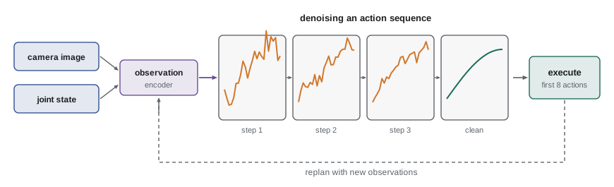
Diffusion models, best known for generating images, learn to reverse a gradual noising process. Training takes a clean sample, adds a random amount of Gaussian noise, and trains a network to predict the noise that was added. Generation starts from pure noise and repeatedly applies the network to remove a little noise at a time until a clean sample emerges. Because generation starts from random noise, different starting points lead to different modes, so the model can represent any number of distinct behaviours.
Diffusion Policy, published by Chi and colleagues in 2023, applies this to robot actions. The network is conditioned on recent observations, typically camera images and joint positions, and denoises a short sequence of future actions rather than an image. Its training loss is simple:
Here \( A \) is a demonstrated action sequence, \( k \) a randomly chosen noise level, \( \bar\alpha_k \) the noise schedule and \( \epsilon \) standard Gaussian noise. At run time, the policy runs perhaps 10 to 100 denoising steps to produce an action sequence, executes the first several actions, then plans again. Diffusion Policy proved markedly better than regression baselines on many manipulation benchmarks, and diffusion or the closely related flow-matching formulation now appears in many robot foundation models, including the π0 family discussed in lesson 11.
Worked problem
Inference time and control rate
A Diffusion Policy network takes 6 ms per denoising step on the robot's computer and uses 16 steps. It predicts 16 future actions at 10 Hz and executes 8 of them before replanning. Can it keep up?
Show solution
- Inference time per plan: \( 16 \times 6 = 96 \) ms.
- Time covered by executed actions: \( 8 / 10 = 0.8 \) s.
- Inference uses about 12 % of each execution window, so it keeps up, and inference can overlap with execution.
Answer: Yes. Fewer denoising steps, distillation or flow matching can cut inference further if a faster control rate is needed.
Action chunking and ACT
The Action Chunking Transformer, ACT, was introduced in 2023 with ALOHA, a low-cost bimanual teleoperation system, by Zhao and colleagues. ACT predicts a chunk of \( k \) future actions at once, for example 100 actions at 50 Hz, two seconds of motion. Chunking reduces the effective horizon of the task by a factor of \( k \), which directly attacks the compounding errors of lesson 8, and it captures the smooth temporal structure of human motion, including pauses that a single-step policy finds confusing. To keep motion smooth when chunks overlap, ACT uses temporal ensembling: at each step it averages the predictions for that step from all recent chunks, weighting older predictions with exponentially decaying weights.
ACT handles multimodality with a conditional variational autoencoder. During training, an encoder compresses the demonstrated action sequence into a small latent style variable, and the decoder, a transformer conditioned on images, joint states and the latent, reconstructs the actions. At test time the latent is set to the prior mean, which selects a single coherent mode rather than an average. With about 50 demonstrations per task, ACT learned fine bimanual skills such as opening a cup lid and inserting a battery, which helped spark the current wave of low-cost imitation-learning research.
| Property | MSE regression | ACT | Diffusion Policy |
|---|---|---|---|
| Output | One action | Chunk of actions | Sequence of actions |
| Multimodality | Averages modes | Latent variable selects a mode | Sampling from noise reaches any mode |
| Inference cost | One forward pass | One forward pass | Many denoising passes |
| Temporal smoothness | Often jittery | Temporal ensembling | Smooth sequences, receding horizon |
| Typical data size per task | Hundreds of demos | About 50 demos | About 100 to 200 demos |
Collecting demonstrations
Imitation learning is only as good as its demonstrations, and how they are collected shapes what can be learned. Common interfaces include kinesthetic teaching, in which the operator physically guides a compliant arm; leader-follower teleoperation, in which the operator moves a small leader arm and a larger follower arm copies it, as in ALOHA; virtual-reality controllers or hand tracking; spacemice and gamepads; and handheld gripper devices that record demonstrations without a robot at all, later mapped onto robot actions. Each trades cost, intuitiveness and fidelity. Leader-follower systems give operators a natural sense of the arm's reach and limits; handheld devices scale data collection beyond the lab but introduce an embodiment gap between the human hand and the robot gripper.
Good practice includes recording all streams with synchronized timestamps; writing a short protocol so operators use a consistent strategy unless diversity is wanted; varying object positions, lighting and distractors deliberately; reviewing and discarding failed or sloppy episodes; and documenting the data with a datasheet that records the robot, sensors, operators, task variations and known gaps. Open tools such as Hugging Face's LeRobot library, at the time of writing, provide standard dataset formats, recording scripts and reference implementations of ACT and Diffusion Policy. Because demonstrations may capture people's faces, voices and homes, collection must also respect privacy law, which lesson 12 maps for Canada and the United States.
Worked problem
Budgeting a demonstration dataset
A team wants 200 demonstrations of a towel-folding task. Each episode takes 45 s, resetting the towel takes 30 s, and about 15 % of episodes are discarded in review. An operator can work productively for 3 hours a day. How many operator-days are needed?
Show solution
- Episodes to record: \( 200 / 0.85 \approx 236 \).
- Time per episode including reset: 75 s, so \( 236 \times 75 = 17{,}700 \) s, about 4.9 hours.
- At 3 productive hours a day: \( 4.9 / 3 \approx 1.6 \), so 2 operator-days.
Answer: About 2 operator-days, plus setup and review time.
# Training ACT or Diffusion Policy with LeRobot (listing only; API at the time of writing)
# lerobot-train \
#   --dataset.repo_id=my_lab/towel_folding \
#   --policy.type=diffusion \
#   --output_dir=outputs/towel_diffusion \
#   --steps=100000 --batch_size=64
from lerobot.datasets.lerobot_dataset import LeRobotDataset
ds = LeRobotDataset("my_lab/towel_folding")
frame = ds[0]
print(frame.keys())   # e.g. observation.images.top, observation.state, action
Common mistakes
MistakeTraining an MSE regression policy on demonstrations with several strategies.
InsteadUse a generative policy, such as a diffusion or chunked latent-variable model, or standardize the strategy.
MistakeExpecting IRL to recover the one true reward.
InsteadIRL is ambiguous; add assumptions such as maximum entropy and validate the learned reward by re-optimizing it.
MistakeRunning a diffusion policy without checking inference latency.
InsteadBudget denoising steps against the control rate, and execute part of each chunk while computing the next.
MistakeKeeping every recorded episode.
InsteadReview and discard failed or inconsistent demonstrations, and document what remains.
MistakeCollecting demonstrations in one fixed arrangement.
InsteadVary object poses, lighting and distractors deliberately during collection.
Summary and key terms
- Inverse RL recovers a reward that explains demonstrations, giving a transferable description of the task.
- IRL is ambiguous; maximum-entropy IRL matches expert feature statistics under a probabilistic model.
- GAIL replaces explicit rewards with a discriminator but still needs many RL steps.
- Regression averages multimodal demonstrations into poor actions.
- Diffusion Policy denoises action sequences conditioned on observations and represents many modes.
- ACT predicts action chunks with a conditional VAE and smooths them by temporal ensembling.
- Demonstration quality, diversity, documentation and privacy determine what imitation can achieve.
- Inverse reinforcement learning
- Inferring a reward function from expert behaviour.
- Maximum-entropy IRL
- IRL that models trajectory probability as proportional to the exponential of return.
- Feature matching
- Adjusting reward weights until model and expert feature statistics agree.
- GAIL
- Generative adversarial imitation learning, using a discriminator as the reward.
- Multimodality
- Several distinct good actions for the same observation.
- Diffusion Policy
- A policy that generates action sequences by iterative denoising.
- Action chunk
- A sequence of future actions predicted at once.
- ACT
- Action Chunking Transformer, a CVAE transformer policy for chunked actions.
- Temporal ensembling
- Averaging overlapping chunk predictions for the same time step.
- Leader-follower teleoperation
- An operator moves a leader device and the robot follower copies it.
Practice problems
Work each problem on paper first, then reveal the answer to check.
Why is IRL ambiguous?
Show answer
Many rewards, including a constant reward, make the same behaviour optimal.
What does the maximum-entropy IRL gradient compare?
Show answer
Expert feature counts with feature counts under the current reward's policy.
What plays the role of the reward in GAIL?
Show answer
The discriminator's output.
Demonstrations go left or right equally. What does MSE regression predict?
Show answer
Their average, straight ahead.
What does a Diffusion Policy network predict during training?
Show answer
The noise added to a demonstrated action sequence.
Why does chunking reduce compounding error?
Show answer
Fewer decisions are made per task, shortening the effective horizon.
What is temporal ensembling?
Show answer
Averaging predictions for the same step from overlapping chunks.
20 steps of 5 ms inference; 8 actions executed at 20 Hz. Fraction of the window used?
Show answer
100 ms out of 400 ms, 25 %.
Name two demonstration interfaces.
Show answer
Kinesthetic teaching, leader-follower arms, VR controllers, spacemice, handheld grippers.
Why write a datasheet for a demonstration dataset?
Show answer
To record the robot, sensors, operators, variations and gaps for later users.
Lesson quiz · 5 questions
Score 60% or more to complete this lesson.
Create a free account to save your progress, take quizzes and earn a certificate.