Statistical quality control

Every process varies: no two shafts, pours of concrete or bottles of product are exactly alike. Statistical quality control distinguishes the ordinary, unavoidable variation of a stable process from variation with a specific, findable cause, such as a worn tool, a new batch of material or an untrained operator, and judges whether a stable process is good enough for its specification. This lesson covers the three main tools. Control charts, invented by Walter Shewhart at Bell Laboratories in the 1920s, monitor a process over time and signal when it changes. Process capability indices compare the natural spread of a stable process with its tolerance. Acceptance sampling decides whether to accept a lot of incoming material from a sample. The lesson draws on the sampling distributions of Lesson 6, the binomial and Poisson distributions of Lesson 4 and the measurement-system ideas of Lesson 2.

Common causes and special causes

Shewhart's key idea was that process variation has two sources. Common-cause variation is the combined effect of many small, ever-present influences: slight differences in raw material, vibration, temperature, measurement error. It is built into the process, and reducing it requires changing the process itself, usually a management decision. Special-cause (assignable-cause) variation comes from a specific event that is not part of the normal process: a broken tool, a mis-set machine, a contaminated batch. It can and should be found and removed by the people running the process.

A process with only common-cause variation is in statistical control: its output is predictable within limits. Two opposite mistakes are costly. Treating common-cause variation as if it had a special cause, adjusting the machine after every slightly high reading, actually increases variation (this is called tampering). Ignoring a special cause lets bad product accumulate. Control charts are designed to tell the two apart.

Control charts for measurements

A control chart plots a statistic from successive samples (subgroups) against time, with a centre line and control limits placed three standard errors either side. For measurements, the usual pair is the \(\bar{X}\) chart, which tracks the process mean, and the R (range) chart, which tracks its spread. Subgroups of n = 4 or 5 consecutive items are taken at regular intervals. From about 20 to 25 subgroups collected while the process seems stable, compute the grand mean \(\bar{\bar{x}}\) and the average range \(\bar{R}\). The limits are

where the constants depend on the subgroup size; for n = 5, \(A_2 = 0.577\), \(D_3 = 0\), \(D_4 = 2.114\), and the process standard deviation is estimated by \(\hat{\sigma} = \bar{R}/d_2\) with \(d_2 = 2.326\). The \(A_2\bar{R}\) term is simply \(3\hat{\sigma}/\sqrt{n}\), three standard errors of the subgroup mean (Lesson 6). Charts with standard deviations instead of ranges (\(\bar{X}\)–s charts) are preferred for larger subgroups, and an individuals chart handles processes where only one measurement is available at a time, such as a daily water quality result.

Reading a control chart

A point outside the control limits is the clearest signal of a special cause: for a stable, normal process, the chance is only 0.27% per point. Patterns inside the limits can also signal a change, and the Western Electric rules are widely used to catch them:

• One point beyond the 3σ limits.
• Two of three consecutive points beyond 2σ on the same side.
• Four of five consecutive points beyond 1σ on the same side.
• Eight consecutive points on the same side of the centre line.

Trends (six points steadily rising or falling) suggest tool wear or drift; cycles suggest shift-to-shift or temperature effects. Each extra rule catches small shifts sooner but adds false alarms, so plants choose a set suited to the cost of each. Performance is measured by the average run length (ARL), the average number of subgroups before a signal: about 370 for a stable process with the 3σ rule alone, but only a few subgroups after a large shift.

import numpy as np

rng = np.random.default_rng(21)
# 30 subgroups of 5 shaft diameters (mm); the process mean shifts up by 0.006 mm after subgroup 20
data = rng.normal(25.002, 0.005, size=(30, 5))
data[20:] += 0.006
xbar, R = data.mean(axis=1), np.ptp(data, axis=1)

# Control limits from the first 20 subgroups (phase I), n = 5: A2 = 0.577, D4 = 2.114, d2 = 2.326
xbb, Rbar = xbar[:20].mean(), R[:20].mean()
UCL, LCL = xbb + 0.577 * Rbar, xbb - 0.577 * Rbar
print(f"Grand mean {xbb:.4f} mm, X-bar limits {LCL:.4f} to {UCL:.4f}, R chart UCL {2.114 * Rbar:.4f}")
out = [i + 1 for i in range(30) if xbar[i] > UCL or xbar[i] < LCL]
print("Subgroups outside the X-bar limits:", out)

# Rule: eight points in a row on the same side of the mean line
side = np.sign(xbar - xbb)
for i in range(7, 30):
    if abs(side[i - 7:i + 1].sum()) == 8:
        print(f"Run of eight on one side ends at subgroup {i + 1}")
        break

sigma = Rbar / 2.326
LSL, USL = 24.975, 25.025
Cp = (USL - LSL) / (6 * sigma)
Cpk = min(USL - xbb, xbb - LSL) / (3 * sigma)
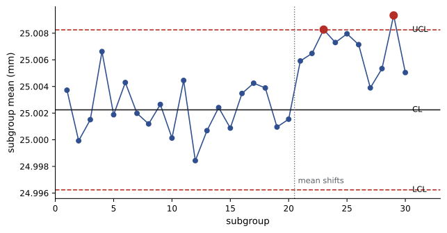
print(f"Estimated sigma {sigma:.5f} mm: Cp = {Cp:.2f}, Cpk = {Cpk:.2f} (before the shift)")

Grand mean 25.0022 mm, X-bar limits 24.9962 to 25.0082, R chart UCL 0.0220
Subgroups outside the X-bar limits: [23, 29]
Run of eight on one side ends at subgroup 28
Estimated sigma 0.00447 mm: Cp = 1.86, Cpk = 1.70 (before the shift)

The limits computed from the stable first period flag points beyond them after the shift, and the run rule also detects the change. Once signalled, the operator looks for the cause (here a tool offset) rather than simply adjusting and moving on. For detecting small, sustained shifts quickly, cumulative sum (CUSUM) and exponentially weighted moving average (EWMA) charts, which accumulate evidence across subgroups, are more sensitive than Shewhart charts.

Control charts for attributes

When items are simply classified as defective or not, a p chart tracks the fraction defective in samples of size n. With average fraction \(\bar{p}\), the limits come from the binomial standard error (Lesson 4):

with a negative lower limit replaced by zero. When counting defects per unit, such as flaws per square metre of sheet or errors per drawing, a c chart uses the Poisson standard deviation, \(\bar{c} \pm 3\sqrt{\bar{c}}\).

Process capability

A process in control is predictable, but it may still not meet its specification. Capability indices compare the process spread with the tolerance between the lower and upper specification limits (LSL and USL):

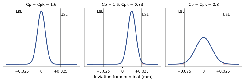
\(C_p\) measures potential capability if the process were centred; \(C_{pk}\) accounts for where the mean actually is, and is the one that predicts defects. A centred process with \(C_p = 1\) produces about 0.27% out of specification (2700 parts per million); \(C_{pk} = 1.33\) corresponds to about 63 ppm, and many industries require at least 1.33 for existing processes and 1.67 for new or safety-critical ones. "Six sigma" quality corresponds to \(C_p = 2\).

Acceptance sampling

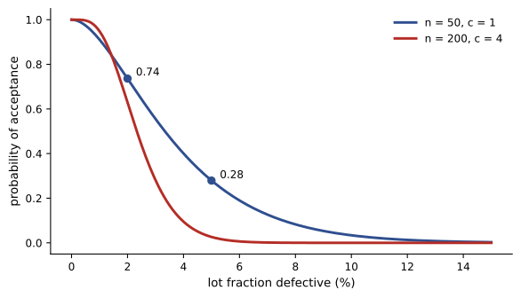
When a lot of purchased parts arrives, inspecting every item may be too costly or, for destructive tests, impossible. A single sampling plan inspects a random sample of n items and accepts the lot if it contains at most c defectives. The plan's operating characteristic (OC) curve gives the probability of acceptance as a function of the lot's true fraction defective p, computed from the binomial distribution: