
STAT-235 · Lesson 6 of 12 · 28 min
Joint variation, error propagation and sampling distributions
Engineering quantities rarely vary alone. The length of an assembly depends on the lengths of all its parts; a computed density depends on a measured mass and a measured volume; the strength and stiffness of timber tend to rise and fall together. This lesson develops the tools for random quantities that act together. It introduces joint distributions, covariance and correlation for random variables, and the rules for the mean and variance of sums, which lead to statistical tolerancing of assemblies. It then shows how uncertainty in measured inputs propagates into a calculated result. Finally it looks at statistics computed from samples as random variables in their own right, and introduces the chi-square, t and F distributions that underlie the confidence intervals and tests of Lessons 7 and 8.
Joint distributions
Two random variables X and Y are described together by a joint distribution: a table of probabilities \(P(X = x, Y = y)\) for discrete variables, or a joint density \(f(x, y)\) whose double integral over a region gives the probability of falling in it (MATH-209) for continuous ones. The distribution of each variable on its own, its marginal distribution, is found by summing or integrating over the other. X and Y are independent when the joint distribution factors into the product of the marginals, so that knowing one tells you nothing about the other.
Worked problem
Defects on two inspection stations
For a part, X is the number of surface defects (0 or 1) and Y the number of dimensional defects (0 or 1). The joint probabilities are P(0, 0) = 0.80, P(0, 1) = 0.05, P(1, 0) = 0.10 and P(1, 1) = 0.05. Are the defect types independent?
Show solution
- Marginals: P(X = 1) = 0.10 + 0.05 = 0.15; P(Y = 1) = 0.05 + 0.05 = 0.10.
- If independent, P(1, 1) would be 0.15 × 0.10 = 0.015.
- The actual P(1, 1) = 0.05 is more than three times larger.
Answer: Not independent: parts with one type of defect are more likely to have the other, suggesting a common cause such as a worn tool or a bad batch of material. That clue is often more useful than either defect rate alone.
Covariance and correlation
The covariance of two random variables measures how they vary together:
It is positive when large values of X tend to go with large values of Y, and negative when they go with small values. Its size depends on the units, so it is usually scaled to the correlation coefficient \(\rho = \text{Cov}(X, Y)/(\sigma_X\sigma_Y)\), which lies between −1 and 1. This is the population version of the sample correlation r of Lesson 1. Independent variables have zero covariance, although zero covariance does not by itself guarantee independence: Y = X² with X symmetric about zero is a standard counterexample.
Sums of random variables and tolerance stack-up
For any constants a and b, the mean of a combination is the combination of the means, \(E[aX + bY] = a\mu_X + b\mu_Y\), and the variance is
For independent variables the covariance term vanishes, and variances (not standard deviations) add. Lesson 4 used this for sums of independent variables; the covariance term matters whenever variables share a common cause, such as parts made from the same bar stock or measurements taken with the same instrument.
The most common engineering application is the tolerance stack-up of an assembly. If n parts with independent dimensions are stacked, the assembly length has standard deviation \(\sqrt{\sigma_1^2 + \cdots + \sigma_n^2}\), which grows only as \(\sqrt{n}\) for equal parts. Worst-case tolerancing, which assumes every part is at its limit in the same direction at once, adds the tolerances directly and so grows as n. For many parts, worst-case design is very conservative and expensive; statistical tolerancing accepts a small, calculated chance of an out-of-tolerance assembly in exchange for much looser part tolerances.
Worked problem
Stacking five spacers
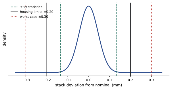
Five spacers, each 10.00 mm nominal with standard deviation 0.02 mm (and parts made to ±0.06 mm, three standard deviations), are stacked in a housing. Compare the worst-case and statistical variation of the stack.
Show solution
- Worst case: 5 × 0.06 = ±0.30 mm.
- Statistical: \(\sigma_{stack} = \sqrt{5} \times 0.02 = 0.0447\) mm, so ±3σ = ±0.134 mm.
- If the housing allows ±0.20 mm, the statistical design meets it with margin, while the worst-case analysis says it fails.
Answer: The ±3σ statistical spread, ±0.13 mm, is less than half the worst-case ±0.30 mm. Statistical tolerancing is valid when the parts really are independent and their processes centred; if all spacers come from one batch with the same offset, the covariance term returns and the worst case becomes more realistic.
Propagation of error
Most engineering results are calculated from several measured inputs, each with its own uncertainty. If \(Y = f(X_1, \ldots, X_k)\) and the inputs are independent with small standard deviations, a first-order Taylor expansion (MATH-209) gives
with the derivatives evaluated at the mean values. For a product of powers, \(Y = cX_1^{a_1}X_2^{a_2}\cdots\), this simplifies to a rule for relative (percentage) uncertainties:
An input raised to a high power dominates the result, so it deserves the most careful measurement.
Worked problem
Uncertainty in a computed power
The power dissipated in a resistor is computed as \(P = I^2R\) from I = 2.00 ± 0.02 A and R = 10.0 ± 0.1 Ω (standard uncertainties). Find P and its uncertainty.
Show solution
- P = 4.00 × 10.0 = 40.0 W.
- Relative uncertainties: 1% for I and 1% for R. With exponents 2 and 1: \(\sigma_P/P = \sqrt{(2 \times 0.01)^2 + (0.01)^2} = 0.0224\).
- \(\sigma_P = 0.0224 \times 40.0 = 0.89\) W.
Answer: P = 40.0 ± 0.9 W. The current contributes four-fifths of the variance because it is squared, so a better ammeter would improve the result far more than a better resistance measurement. Measurement standards (the GUM, the international Guide to the Expression of Uncertainty in Measurement) formalize exactly this procedure.
When the function is strongly nonlinear or the uncertainties are large, the first-order formula can mislead. Monte Carlo simulation, sampling the inputs and computing the result many times (MATH-300), handles any function and also gives the shape of the output distribution.
Statistics as random variables
A statistic such as the sample mean or the sample standard deviation is computed from random data, so it is itself a random variable with its own sampling distribution: a different sample would give a different value. Lesson 4 showed that the sample mean has mean μ and standard deviation \(\sigma/\sqrt{n}\) (the standard error), and is approximately normal for large n by the central limit theorem. Three further distributions describe other statistics from normal samples.
The chi-square distribution
For a random sample of size n from a normal population, the scaled sample variance follows a chi-square distribution with n − 1 degrees of freedom:
A chi-square variable with ν degrees of freedom is the sum of ν squared independent standard normal variables; it is positive and skewed right, with mean ν and variance 2ν. One degree of freedom is lost because the deviations are measured from the sample mean rather than the true mean, which is also why the sample variance divides by n − 1. This distribution gives confidence intervals and tests for a variance (Lesson 8), important when consistency matters as much as the average, as for the fill weight of packages or the thickness of a coating.
The t distribution
When σ is unknown and estimated by s, the standardized sample mean follows Student's t distribution with n − 1 degrees of freedom:
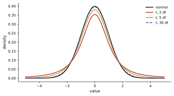
The t distribution is symmetric like the normal but has heavier tails, reflecting the extra uncertainty of estimating σ from a small sample. As n grows it approaches the standard normal. W. S. Gosset derived it in 1908 while working on small samples at the Guinness brewery in Dublin, publishing under the pen name "Student". For small samples the difference matters, as the simulation below shows.
import numpy as np
from scipy import stats

rng = np.random.default_rng(5)
mu, sigma, n, reps = 50.0, 2.0, 5, 100_000
samples = rng.normal(mu, sigma, size=(reps, n))
xbar = samples.mean(axis=1)
s = samples.std(axis=1, ddof=1)

print(f"SD of sample means: {xbar.std():.3f} (theory sigma/sqrt(n) = {sigma / np.sqrt(n):.3f})")
chi = (n - 1) * s**2 / sigma**2
print(f"(n-1)s^2/sigma^2: mean {chi.mean():.2f}, variance {chi.var():.2f} (chi-square, 4 df: 4 and 8)")

# 95% intervals for the mean using s: with z = 1.96 versus t with n - 1 degrees of freedom
z, t = 1.96, stats.t.ppf(0.975, n - 1)
half_z, half_t = z * s / np.sqrt(n), t * s / np.sqrt(n)
cover_z = np.mean(np.abs(xbar - mu) <= half_z)
cover_t = np.mean(np.abs(xbar - mu) <= half_t)
print(f"t multiplier for 4 df: {t:.3f}")
print(f"Coverage using z = 1.96: {cover_z:.3f}; using t: {cover_t:.3f}")SD of sample means: 0.893 (theory sigma/sqrt(n) = 0.894) (n-1)s^2/sigma^2: mean 3.99, variance 7.91 (chi-square, 4 df: 4 and 8) t multiplier for 4 df: 2.776 Coverage using z = 1.96: 0.877; using t: 0.950
The simulation confirms the theory: the sample means have standard deviation σ/√n, the scaled variances have the mean and variance of a chi-square with 4 degrees of freedom, and an interval built with 1.96 instead of the t multiplier 2.776 covers the true mean only 88% of the time instead of the promised 95%.
The F distribution
The ratio of two independent sample variances, each divided by its population variance, follows an F distribution with two degrees-of-freedom parameters:
It is used to compare the variability of two processes (Lesson 8) and, most importantly, in the analysis of variance (Lesson 9), which compares several means by comparing variances.
Common mistakes
MistakeAdding standard deviations of independent parts.
InsteadAdd variances; the standard deviation of a sum grows as the square root.
MistakeIgnoring correlation when inputs share a common cause.
InsteadInclude the covariance term 2ab Cov(X, Y).
MistakeAssuming zero correlation means independence.
InsteadZero covariance rules out only linear association.
MistakeGiving every input equal attention in an uncertainty budget.
InsteadInputs with large exponents or sensitivities dominate; measure them best.
MistakeUsing z = 1.96 with s from a small sample.
InsteadUse the t multiplier with n − 1 degrees of freedom.
Summary and key terms
- Joint distributions describe variables together; independence means the joint distribution factors into the marginals.
- Covariance and correlation measure linear association between random variables.
- Var(aX + bY) = a²σ_X² + b²σ_Y² + 2ab Cov(X, Y); independent variances add.
- Statistical tolerancing grows as √n, worst-case as n.
- Propagation of error: σ_Y² ≈ Σ(∂f/∂xᵢ)²σᵢ²; for products of powers, relative variances add, weighted by squared exponents.
- (n − 1)S²/σ² is chi-square with n − 1 degrees of freedom; (X̄ − μ)/(S/√n) is t with n − 1.
- The F distribution describes ratios of variances and underlies the analysis of variance.
- Joint distribution
- The probability distribution of two or more random variables together.
- Marginal distribution
- The distribution of one variable, obtained by summing or integrating out the others.
- Covariance
- E[(X − μ_X)(Y − μ_Y)], a measure of joint variation.
- Correlation coefficient
- Covariance divided by the product of standard deviations.
- Tolerance stack-up
- The accumulation of part variations in an assembly.
- Statistical tolerancing
- Combining part tolerances by adding variances.
- Propagation of error
- Estimating the uncertainty of a computed result from input uncertainties.
- Sampling distribution
- The distribution of a statistic over repeated samples.
- Chi-square distribution
- The distribution of a sum of squared standard normal variables.
- t distribution
- The distribution of a standardized mean when σ is estimated by s.
- F distribution
- The distribution of a ratio of two scaled independent variances.
Practice problems
Work each problem on paper first, then reveal the answer to check.
X and Y are independent with σ_X = 3 and σ_Y = 4. Find the standard deviation of X + Y and of X − Y.
Show answer
Both 5.
If Cov(X, Y) = 6 in that problem, find the standard deviation of X + Y.
Show answer
√(9 + 16 + 12) = 6.08.
Ten parts each with σ = 0.01 mm are stacked. What is the stack σ?
Show answer
0.0316 mm.
Compare worst-case and ±3σ statistical tolerance for ten parts each ±0.03 mm (3σ).
Show answer
Worst case ±0.30 mm; statistical ±0.095 mm.
A cube has side 50.0 ± 0.1 mm. Find the relative uncertainty in its volume.
Show answer
3 × 0.2% = 0.6%.
Density ρ = m/V with m uncertain by 0.5% and V by 1.2%. Relative uncertainty of ρ?
Show answer
√(0.25 + 1.44)% = 1.3%.
What are the mean and variance of a chi-square variable with 10 degrees of freedom?
Show answer
10 and 20.
Find the 95% t multiplier for n = 10.
Show answer
t₀.₀₂₅,₉ = 2.262.
Why does the t distribution have heavier tails than the normal?
Show answer
It accounts for the extra uncertainty of estimating σ from the sample.
Two samples of sizes 8 and 12 are compared for variance. What are the F degrees of freedom?
Show answer
7 and 11.
Lesson quiz · 5 questions
Score 60% or more to complete this lesson.
Create a free account to save your progress, take quizzes and earn a certificate.