
ECON-101 · Lesson 4 of 12 · 30 min
Elasticity
The law of demand tells us that buyers purchase less when prices rise, but not how much less. For many decisions, the size of the response is what matters. A transit authority considering a fare increase needs to know whether ridership will fall a little or a lot; a government taxing cigarettes wants to know whether the tax will mainly raise revenue or mainly reduce smoking; a farmer wants to know whether a bumper harvest will raise or lower her income. Elasticity measures how responsive one variable is to a change in another. BUS-220 lesson 9 used price elasticity to set prices for a product; this lesson develops the concept more fully, including income and cross-price elasticities and the elasticity of supply, and shows why elasticity determines who bears the burden of a tax.
Price elasticity of demand
The price elasticity of demand is the percentage change in quantity demanded divided by the percentage change in price. Because price and quantity demanded move in opposite directions, the result is negative; by convention, economists usually report its absolute value. If a 10 % rise in the price of gasoline reduces the quantity demanded by 2 %, the price elasticity of demand is 0.2.
Demand is elastic when \( E_d > 1 \): quantity responds more than proportionally to price. It is inelastic when \( E_d < 1 \): quantity responds less than proportionally. It is unit elastic when \( E_d = 1 \). Two limiting cases help intuition. Perfectly inelastic demand (\( E_d = 0 \)) means buyers purchase the same quantity whatever the price, as might be roughly true for a life-saving drug with no substitutes; the demand curve is vertical. Perfectly elastic demand (\( E_d = \infty \)) means buyers will purchase none at all if the price rises even slightly above a given level, as for one farmer's wheat in a large world market; the demand curve is horizontal.
The midpoint method
Percentage changes depend on the starting point. If the price rises from $4 to $5, that is a 25 % increase; if it falls from $5 to $4, that is a 20 % decrease. To get the same elasticity in either direction, economists use the midpoint (or arc) method, which divides each change by the average of the starting and ending values.
Worked problem
Transit fares
A city raises the adult transit fare from $3.25 to $3.75, and weekday boardings fall from 420,000 to 395,000. Calculate the price elasticity of demand using the midpoint method, and say whether demand is elastic or inelastic.
Show solution
- Percentage change in quantity: (395,000 − 420,000) ÷ 407,500 = −6.13 %.
- Percentage change in price: (3.75 − 3.25) ÷ 3.50 = +14.29 %.
- Elasticity: |−6.13 ÷ 14.29| = 0.43.
Answer: Demand is inelastic (0.43). Ridership falls, but proportionally less than the fare rises, so fare revenue increases. Studies of North American transit typically find short-run fare elasticities between about 0.2 and 0.5, larger in the long run as people adjust where they live and how they commute.
What determines price elasticity
Several factors determine how elastic demand is. The most important is the availability of close substitutes: demand for a particular brand of cola is very elastic because other colas are close substitutes, while demand for soft drinks as a category is less elastic, and demand for beverages in general less elastic still. This shows that elasticity depends on how broadly the market is defined. Necessities tend to have inelastic demand and luxuries elastic demand, though what counts as a necessity varies by person and over time. Goods that take up a large share of the budget, such as housing and cars, tend to have more elastic demand than goods that take a tiny share, such as salt or matches, because a price change matters more to the buyer. And time matters: demand is usually more elastic in the long run, because people need time to find substitutes. When gasoline prices rise, people initially have little choice but to keep driving, but over several years they buy more efficient cars, move closer to work or switch to transit.
| Good or service | Typical estimated price elasticity | Interpretation |
|---|---|---|
| Cigarettes (adults, short run) | 0.3 to 0.5 | Inelastic: addictive, few substitutes |
| Gasoline (short run) | 0.1 to 0.3 | Very inelastic in the short run |
| Gasoline (long run) | 0.5 to 0.8 | More elastic as people adjust |
| Electricity (residential, short run) | 0.1 to 0.3 | Inelastic |
| Restaurant meals | 1.5 to 2.5 | Elastic: home cooking is a substitute |
| A particular brand of cereal | Above 3 | Very elastic: many close substitutes |
Elasticity and total revenue
Elasticity tells a seller what will happen to total revenue (price times quantity) when the price changes. If demand is inelastic, a price increase raises total revenue, because the percentage fall in quantity is smaller than the percentage rise in price. If demand is elastic, a price increase reduces total revenue. If demand is unit elastic, total revenue does not change. This is called the total revenue test.
| If demand is | A price increase | A price decrease |
|---|---|---|
| Elastic (\( E_d > 1 \)) | Lowers total revenue | Raises total revenue |
| Unit elastic (\( E_d = 1 \)) | Leaves total revenue unchanged | Leaves total revenue unchanged |
| Inelastic (\( E_d < 1 \)) | Raises total revenue | Lowers total revenue |
Along a straight-line demand curve, elasticity is not constant even though the slope is. At high prices and low quantities, a given change in price is a small percentage of the price but a large percentage of the quantity, so demand is elastic. At low prices and high quantities the reverse holds, so demand is inelastic. Total revenue is greatest at the midpoint of the line, where elasticity equals one. The following code shows this for a demand curve \( Q = 100 - 10P \).
# Elasticity and total revenue along the linear demand curve Q = 100 - 10P
def quantity(p):
    return 100 - 10 * p
print(" price  qty  revenue  point elasticity")
for p in [9, 8, 7, 6, 5, 4, 3, 2, 1]:
    q = quantity(p)
    e = 10 * p / q            # |dQ/dP| * P/Q
    kind = "elastic" if e > 1 else ("unit" if abs(e - 1) < 1e-9 else "inelastic")
print(f"{p:5} {q:4} {p * q:7} {e:6.2f} {kind}") price qty revenue point elasticity
9 10 90 9.00 elastic
8 20 160 4.00 elastic
7 30 210 2.33 elastic
6 40 240 1.50 elastic
5 50 250 1.00 unit
4 60 240 0.67 inelastic
3 70 210 0.43 inelastic
2 80 160 0.25 inelastic
1 90 90 0.11 inelastic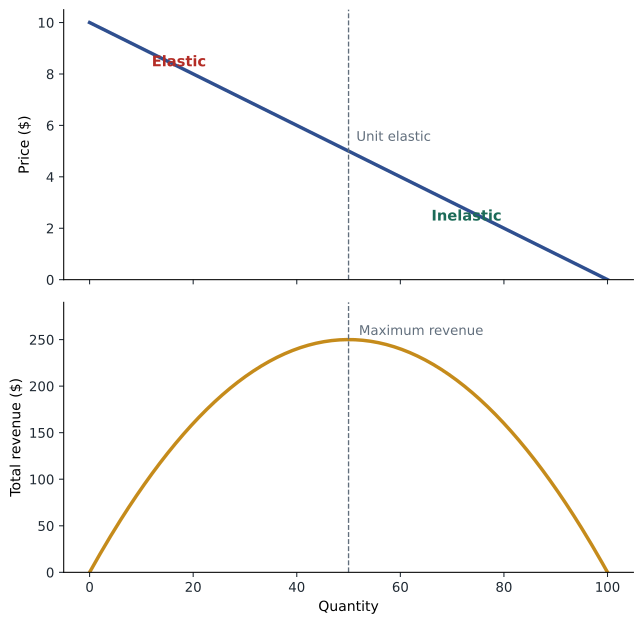
The total revenue test explains a farm paradox. Demand for staple crops is inelastic, so a bumper harvest that shifts supply to the right lowers the price by a larger percentage than it raises the quantity sold, and farmers' total revenue falls. A drought that cuts supply can raise total farm revenue, although individual farmers whose crops failed are badly hurt. This is one reason governments in both Canada and the United States run farm income stabilization programs such as AgriStability and crop insurance.
Income elasticity and cross-price elasticity
Elasticity can measure responsiveness to any variable. The income elasticity of demand is the percentage change in quantity demanded divided by the percentage change in income. It is positive for normal goods and negative for inferior goods. Normal goods with an income elasticity greater than one are often called luxuries: spending on them rises more than proportionally as income grows. Foreign travel, restaurant meals and new cars typically have income elasticities above one; food eaten at home and basic clothing have elasticities between zero and one. This explains why the share of household spending on food falls as countries grow richer, a pattern known as Engel's law.
The cross-price elasticity of demand is the percentage change in the quantity demanded of one good divided by the percentage change in the price of another. It is positive for substitutes, because a rise in the price of tea increases the quantity of coffee demanded, and negative for complements, because a rise in the price of printers reduces the quantity of ink demanded. Competition authorities use cross-price elasticities to define markets in merger cases: if consumers would readily switch from one product to another when its price rises, the two products are probably in the same market, a topic we return to in lesson 11.
Worked problem
Using income and cross-price elasticities
A ski resort estimates that the income elasticity of demand for lift tickets is 1.6 and the cross-price elasticity with respect to the price of airline tickets is −0.4. Next season, average incomes of its customers are expected to rise 3 % and airfares to rise 10 %. Predict the change in lift tickets demanded, holding the lift price constant.
Show solution
- Income effect: 1.6 × 3 % = +4.8 %.
- Airfare effect: −0.4 × 10 % = −4.0 % (complements: people fly to ski).
- Combined: +4.8 % − 4.0 % = +0.8 %.
Answer: Lift ticket demand is predicted to rise by about 0.8 %. Lift tickets behave as a luxury, and air travel is a complement.
Price elasticity of supply
The price elasticity of supply is the percentage change in quantity supplied divided by the percentage change in price. Supply is elastic when producers can easily expand output, for example when spare capacity exists, inputs are readily available and production is quick. Supply is inelastic when output is hard to change, as for land in a city center, tickets to a sold-out arena or, in the short run, apartments, which take years to plan and build. Time is again crucial: supply is usually much more elastic in the long run than in the short run. Housing supply is a key example; studies find that metropolitan areas with tight land-use restrictions, such as Vancouver, Toronto, San Francisco and Boston, have much less elastic housing supply than places with abundant land and permissive rules, such as Calgary or Houston, and accordingly see larger price increases when demand rises.
Elasticity and the burden of a tax
Elasticity also determines who really pays a tax. The legal obligation to remit a tax, its statutory incidence, says little about who bears its burden, its economic incidence. When a tax is imposed on a good, it drives a wedge between the price buyers pay and the price sellers receive. The side of the market that is less elastic bears more of the burden, because it is less able to escape by changing its behavior. If demand is very inelastic, as for cigarettes, most of a cigarette tax is passed on to smokers in higher prices. If supply is very inelastic, as for land, most of a tax falls on owners. A useful approximation is that the share of a tax borne by buyers is \( E_s / (E_s + E_d) \).
Worked problem
Who pays a fuel tax
Suppose the short-run price elasticity of demand for gasoline is 0.2 and the elasticity of supply to a regional market is 1.8. A government raises the fuel excise tax by 10 cents per liter. Approximately how much of the tax is passed on to drivers?
Show solution
- Buyers' share = 1.8 ÷ (1.8 + 0.2) = 0.9.
- Sellers' share = 0.2 ÷ 2.0 = 0.1.
- Pass-through: about 0.9 × 10 cents = 9 cents per liter.
Answer: Drivers pay about 9 of the 10 cents in the short run. The illustrative elasticities match the common finding that fuel taxes are largely passed through to pump prices. Lesson 6 develops tax incidence with diagrams.
This logic explains why governments often tax goods with inelastic demand: such taxes raise substantial revenue without greatly changing behavior. But if the aim of a tax is to change behavior, as with taxes on tobacco or sugary drinks, inelastic demand means the tax must be large to have much effect. The same principle applies to payroll taxes: whatever the legal split between employers and employees, economists find that much of the burden falls on workers through lower wages, because labor supply tends to be less elastic than labor demand.
Common mistakes
MistakeA steep demand curve always means inelastic demand.
InsteadElasticity depends on percentages, not slope; along a straight line, elasticity changes from elastic to inelastic.
MistakeRaising the price always raises revenue.
InsteadA price increase raises revenue only when demand is inelastic.
MistakeThe party that legally pays a tax bears its burden.
InsteadEconomic incidence depends on elasticities; the less elastic side bears more.
MistakeIncome elasticity is always positive.
InsteadIt is negative for inferior goods.
MistakeElasticities are fixed numbers.
InsteadThey vary with time horizon, market definition, price level and context.
Summary and key terms
- Price elasticity of demand is the percentage change in quantity demanded divided by the percentage change in price, reported as an absolute value.
- The midpoint method gives the same elasticity whichever direction the change goes.
- Demand is more elastic with close substitutes, for luxuries, for large budget shares and in the long run.
- With inelastic demand a price rise raises total revenue; with elastic demand it lowers revenue.
- Elasticity varies along a straight-line demand curve; revenue peaks at unit elasticity.
- Income elasticity separates normal goods (positive) from inferior goods (negative); cross-price elasticity separates substitutes (positive) from complements (negative).
- Supply elasticity reflects how easily output can expand, and rises with time.
- The less elastic side of the market bears more of a tax.
- Price elasticity of demand
- The responsiveness of quantity demanded to a change in price.
- Elastic demand
- Demand for which the elasticity exceeds one.
- Inelastic demand
- Demand for which the elasticity is less than one.
- Midpoint method
- Calculating percentage changes relative to the average of the starting and ending values.
- Total revenue
- Price multiplied by quantity sold.
- Income elasticity of demand
- The responsiveness of quantity demanded to a change in income.
- Cross-price elasticity
- The responsiveness of quantity demanded of one good to the price of another.
- Price elasticity of supply
- The responsiveness of quantity supplied to a change in price.
- Statutory incidence
- Who is legally required to pay a tax.
- Economic incidence
- Who actually bears the burden of a tax.
Practice problems
Work each problem on paper first, then reveal the answer to check.
Price rises from $10 to $12; quantity falls from 500 to 400. Midpoint elasticity?
Show answer
22.2 % ÷ 18.2 % ≈ 1.22, elastic.
Will raising price in the previous question raise or lower revenue?
Show answer
Lower: revenue falls from $5,000 to $4,800.
Why is demand for a specific brand more elastic than for the product category?
Show answer
Other brands are close substitutes.
Income rises 5 % and quantity of bus trips falls 2 %. Income elasticity and good type?
Show answer
−0.4; an inferior good.
The price of hot dogs rises 10 % and buns sold fall 6 %. Cross-price elasticity?
Show answer
−0.6; complements.
Why is housing supply more elastic in Houston than in Vancouver?
Show answer
More available land and fewer land-use restrictions.
If E_d = 0.5 and E_s = 1.5, what share of a tax do buyers bear?
Show answer
1.5 ÷ 2.0 = 75 %.
Why might a bumper harvest reduce farm income?
Show answer
Demand is inelastic, so the price falls proportionally more than quantity rises.
Why is demand more elastic in the long run?
Show answer
Buyers have time to find substitutes and change habits.
Portfolio task: estimate the elasticity of demand for something you buy by asking how your purchases would change if its price rose 20 %.
Show answer
Answers vary; should calculate a percentage response and classify it.
Lesson quiz · 5 questions
Score 60% or more to complete this lesson.
Create a free account to save your progress, take quizzes and earn a certificate.