
ECON-101 · Lesson 9 of 12 · 27 min
Perfect competition
Lessons 3 to 6 assumed competitive markets without looking closely at the firms inside them. This lesson does. Perfect competition is a model of an industry with so many sellers of an identical product that no single firm can influence the price. Few industries meet every condition exactly, but agricultural commodities such as wheat and canola, some financial markets, and many small-business sectors come close. The model matters for two reasons: it explains how prices and output are determined in competitive industries, and it provides the efficiency benchmark against which monopoly and oligopoly, in lessons 10 and 11, are judged.
The conditions of perfect competition
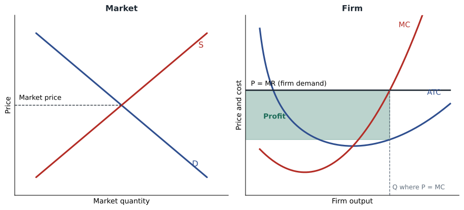
A perfectly competitive market has four features. There are many buyers and sellers, each small relative to the market. The product is homogeneous: buyers regard every seller's product as identical, so they have no reason to pay more to one seller than another. There is free entry and exit in the long run: firms can start up or shut down without special legal or technical barriers. And buyers and sellers have good information about prices and products. Under these conditions, each firm is a price taker: it can sell as much as it wants at the market price, but nothing at a higher price, because buyers would go to other sellers. The demand curve facing an individual firm is therefore horizontal at the market price, even though the market demand curve slopes downward.
A Saskatchewan wheat farmer illustrates price taking. Her harvest, however large, is a tiny fraction of the world wheat market. She can sell her whole crop at the going price, and if she asked more, grain buyers would simply buy elsewhere. Her decisions are about how much to grow and how to grow it, not what price to charge.
Revenue for a price taker
For a price-taking firm, total revenue is price times quantity, and marginal revenue (MR), the extra revenue from selling one more unit, equals the price, because the firm can sell additional units without lowering its price. Average revenue also equals the price.
Choosing output to maximize profit
A firm maximizes profit by producing the quantity at which marginal revenue equals marginal cost. If MR exceeds MC, producing one more unit adds more to revenue than to cost, so profit rises; if MC exceeds MR, cutting output raises profit. For a price taker, MR equals the price, so the profit-maximizing rule becomes: produce where \( P = MC \), on the rising part of the marginal cost curve. This rule applies to every firm, competitive or not, in the form \( MR = MC \); what is special about perfect competition is that MR equals price.
Once the firm has chosen its output, its profit is \( (P - ATC) \times Q \). If the price is above average total cost at that output, the firm makes an economic profit; if it is below, the firm makes a loss.
# Profit-maximizing output for a price-taking farm (illustrative numbers)
# Output in hundreds of tonnes; fixed cost $30,000; variable costs rise with diminishing returns
fixed = 30_000
vc = {0: 0, 1: 22_000, 2: 40_000, 3: 56_000, 4: 74_000, 5: 96_000, 6: 124_000, 7: 160_000}
for price_per_100t in (30_000, 23_000, 17_000):
    best = max(vc, key=lambda q: price_per_100t * q - fixed - vc[q])
    profit = price_per_100t * best - fixed - vc[best]
    sign = "-" if profit < 0 else ""
    avc = f"${vc[best] / best:,.0f}" if best else "n/a (shut down)"
    print(f"price ${price_per_100t:,} per 100 t: produce {best} (00 t), profit {sign}${abs(profit):,}, AVC {avc}")
print("marginal cost of each extra 100 t:", [vc[q] - vc[q - 1] for q in range(1, 8)])price $30,000 per 100 t: produce 6 (00 t), profit $26,000, AVC $20,667 price $23,000 per 100 t: produce 5 (00 t), profit -$11,000, AVC $19,200 price $17,000 per 100 t: produce 0 (00 t), profit -$30,000, AVC n/a (shut down) marginal cost of each extra 100 t: [22000, 18000, 16000, 18000, 22000, 28000, 36000]
At a price of $30,000 per hundred metric tons, the farm produces 600 metric tons, where the marginal cost of the last hundred metric tons ($28,000) is just below the price and the next hundred would cost $36,000, and earns a profit of $26,000. At $23,000 it produces 500 metric tons and loses $11,000, because the price is below average total cost. But producing still beats shutting down, which would lose the full $30,000 of fixed cost. At $17,000 the best choice is to produce nothing: the best positive output, 300 metric tons, would lose $35,000, more than the $30,000 of fixed cost it loses by shutting down. The next section explains this shutdown rule.
The shutdown decision
In the short run, a firm making a loss must decide whether to keep operating or shut down temporarily. If it shuts down, it earns no revenue but still pays its fixed costs, which are sunk in the short run. If it operates, it earns revenue and pays both fixed and variable costs. It should operate if revenue covers variable costs, because then it earns something toward its fixed costs and loses less than by shutting down. The short-run shutdown rule is therefore: shut down if the price is below average variable cost at the best output.
In the long run, when fixed costs can be avoided by leaving the industry, a firm exits if the price is below average total cost, because it cannot cover all its costs. The short-run supply curve of a competitive firm is therefore the part of its marginal cost curve above the minimum of average variable cost. This is the deep reason the market supply curve slopes upward: it is the sum of firms' marginal cost curves.
Worked problem
Applying the shutdown rule
A ski hill has fixed costs of $1.2 million a season (loans, insurance, lift maintenance) and expects variable costs of $2.0 million if it opens (staff, snowmaking, energy). In a poor snow year it expects revenue of $2.3 million if it opens. Should it open? What if revenue would be only $1.8 million?
Show solution
- If it opens with $2.3 million revenue: profit = $2.3m − $1.2m − $2.0m = −$0.9 million.
- If it stays closed: loss = fixed costs = −$1.2 million.
- Opening loses $0.3 million less, because revenue exceeds variable cost by $0.3 million.
- With $1.8 million revenue: opening loses $1.4 million, more than the $1.2 million from staying closed.
Answer: Open when revenue is $2.3 million, because it covers variable costs; stay closed when revenue is $1.8 million. If poor seasons persist, the owners should consider exiting in the long run, since revenue does not cover total cost.
Long-run equilibrium: entry and exit
Free entry and exit drive the long-run outcome. Suppose the market price is high enough that firms earn economic profits. Those profits attract new firms, and existing firms expand. Market supply shifts right, the price falls, and profits shrink. Entry continues until economic profits are zero. Conversely, if firms are making losses, some exit, supply shifts left, the price rises and losses shrink until the remaining firms earn zero economic profit. In long-run equilibrium, then, the price equals the minimum of average total cost, and each firm earns a normal profit.
This result has striking implications. First, competitive firms produce at the lowest possible average cost, at the bottom of their ATC curves: this is productive efficiency. Second, because price equals marginal cost, the value buyers place on the last unit equals its cost of production: this is allocative efficiency, the condition for maximizing total surplus from lesson 5. Third, profits in a competitive industry are temporary signals: they attract resources into industries where consumers want more output and drive them out of industries where consumers want less. Zero economic profit does not mean that owners earn nothing; it means they earn exactly what they could earn elsewhere.
| Condition | Short run | Long run |
|---|---|---|
| Firm's output rule | Produce where P = MC if P ≥ minimum AVC | Produce where P = MC = minimum ATC |
| Profit | Can be positive, zero or negative | Zero economic profit (normal profit) |
| Number of firms | Fixed | Adjusts through entry and exit |
| Efficiency | Allocatively efficient (P = MC) | Allocatively and productively efficient |
The long-run supply curve
What does the industry's long-run supply curve look like? If the industry can expand without affecting input prices, new firms can enter with the same costs as existing ones, and the long-run supply curve is horizontal at the minimum of average total cost: a constant-cost industry. An increase in demand raises the price temporarily, but entry brings it back down. If expansion bids up the prices of scarce inputs, such as specialized labor or suitable land, costs rise as the industry grows, and the long-run supply curve slopes upward: an increasing-cost industry. Some industries even become cheaper as they grow, because a larger industry supports specialized suppliers and a pool of skilled workers: a decreasing-cost industry.
Worked problem
Entry after a demand increase
The market for a commodity is in long-run equilibrium at $8 per unit, the minimum ATC of each identical firm, with 100 firms each producing 1,000 units. Demand increases, and the short-run price rises to $11. Describe what happens in a constant-cost industry, and find the long-run price and number of firms if long-run quantity demanded at $8 is now 130,000 units.
Show solution
- At $11, existing firms earn economic profits, attracting entry.
- Entry shifts supply right until the price returns to minimum ATC, $8.
- At $8, quantity demanded is 130,000 units, and each firm produces 1,000.
- Number of firms: 130,000 ÷ 1,000 = 130.
Answer: In the long run the price returns to $8, and 30 new firms have entered. The extra demand is met by more firms, not higher prices.
How well does the model fit?
Real markets depart from perfect competition in many ways. Products are often differentiated by brand, location or quality; information is imperfect; entry can be costly; and many industries have a few large firms. Yet the model's predictions about entry, exit and the erosion of profits hold widely. When a new food trend, such as bubble tea or poke bowls, proves profitable, new shops open quickly and margins fall. When demand falls, as for video rental stores after streaming arrived, firms exit. The model also explains why many economists see competition as the best protection for consumers: it pushes prices toward cost and rewards firms that cut costs or improve products. Farm policy illustrates a different point: because agricultural markets are close to competitive and demand is inelastic, prices and incomes are volatile, which is why both Canada and the United States run programs to stabilize farm incomes.
Common mistakes
MistakeA competitive firm should charge more than the market price if its costs are high.
InsteadA price taker cannot sell anything above the market price; it can only choose how much to produce.
MistakeA firm should shut down whenever it makes a loss.
InsteadIn the short run it should operate if price covers average variable cost, because that reduces the loss below its fixed cost.
MistakeZero economic profit means the owners earn nothing.
InsteadIt means they earn a normal return, equal to what their resources could earn elsewhere.
MistakeProfit is maximized where average cost is lowest.
InsteadProfit is maximized where marginal revenue equals marginal cost, which need not be at minimum ATC in the short run.
MistakeHigh profits in a competitive industry last indefinitely.
InsteadEntry erodes economic profits until they reach zero in the long run.
Summary and key terms
- Perfect competition has many small firms, a homogeneous product, free entry and exit, and good information.
- Each firm is a price taker facing a horizontal demand curve; marginal revenue equals price.
- All firms maximize profit where MR = MC; for a price taker, P = MC.
- Operate in the short run if price is at least minimum AVC; exit in the long run if price is below minimum ATC.
- The firm's short-run supply curve is its MC curve above minimum AVC.
- Entry and exit drive economic profit to zero in the long run, with price equal to minimum ATC.
- Long-run competitive equilibrium is both productively and allocatively efficient.
- Long-run industry supply is horizontal for constant-cost industries and upward-sloping for increasing-cost industries.
- Perfect competition
- A market with many firms selling identical products with free entry and exit.
- Price taker
- A firm that cannot influence the market price.
- Marginal revenue
- The extra revenue from selling one more unit.
- Profit-maximizing rule
- Produce where marginal revenue equals marginal cost.
- Shutdown rule
- Stop producing in the short run if price is below average variable cost.
- Exit
- Leaving an industry in the long run when price is below average total cost.
- Productive efficiency
- Producing at the lowest possible average cost.
- Allocative efficiency
- Producing the quantity where price equals marginal cost.
- Constant-cost industry
- An industry whose long-run supply curve is horizontal.
- Increasing-cost industry
- An industry whose costs rise as it expands, giving an upward-sloping long-run supply curve.
Practice problems
Work each problem on paper first, then reveal the answer to check.
Why is the demand curve facing a competitive firm horizontal?
Show answer
It is tiny relative to the market and sells an identical product, so it can sell any amount at the market price but nothing above it.
Price is $40. MC of the 100th unit is $36 and of the 101st is $44. How many units?
Show answer
100.
At that output ATC is $45. Profit or loss?
Show answer
Loss of $5 × 100 = $500.
AVC at that output is $32. Should the firm operate in the short run?
Show answer
Yes, price exceeds AVC.
What happens in the long run if this situation persists?
Show answer
Some firms exit, raising the price, or this firm exits.
What is the firm's short-run supply curve?
Show answer
Its MC curve above minimum AVC.
Why are long-run economic profits zero in perfect competition?
Show answer
Entry and exit adjust supply until price equals minimum ATC.
Define allocative efficiency.
Show answer
Producing where price equals marginal cost.
A market is at $5 with 200 firms each producing 500 units. Demand rises so that 120,000 units are demanded at $5. In a constant-cost industry, how many firms in the long run?
Show answer
240.
Portfolio task: choose an industry near perfect competition and describe a recent episode of entry or exit and its effect on prices.
Show answer
Answers vary; should link profit signals to entry or exit.
Lesson quiz · 5 questions
Score 60% or more to complete this lesson.
Create a free account to save your progress, take quizzes and earn a certificate.