Modeling case studies and course project

The previous eleven lessons built a toolkit: first-order methods and phase lines, linear equations of every order, oscillators, boundary value and eigenvalue problems, Laplace transforms and transfer functions, linear and nonlinear systems, and partial differential equations. In practice, an engineer is rarely told which tool to use. The work starts with a physical situation and a question, and the skill lies in turning that into a model, choosing a method, checking the answer and deciding what it means. This lesson works through three case studies that each draw on several lessons: protecting a building from earthquake shaking, preventing thermal runaway in a battery cell, and finding how deep to bury a water main so that it does not freeze. It then sets out the course project and looks ahead to the courses that build on this one.

Case study 1: base isolation of a building

In an earthquake, the ground moves and the building is shaken from below. If the dominant ground frequency is close to a natural frequency of the building, the response is amplified, as Lesson 5 showed for forced vibration. Base isolation places flexible bearings (laminated rubber or sliding pendulum bearings) between the building and its foundation, making the whole structure behave like a single mass on a soft, damped spring with a long natural period.

Model the building as a rigid mass m on isolators of stiffness k and damping c. With ground displacement \(y = Y\sin\omega t\) and building displacement x, Newton's law gives \(m\ddot{x} + c(\dot{x} - \dot{y}) + k(x - y) = 0\). The transfer function from ground to building, evaluated at \(s = i\omega\) (Lesson 8), gives the transmissibility, the ratio of building to ground motion amplitudes:

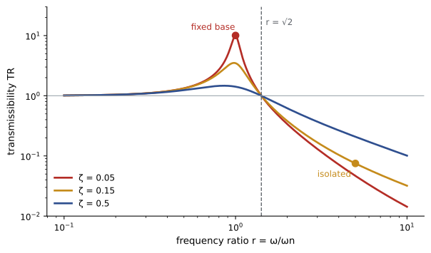
The model uses Lessons 5 and 8, and a real design adds the multi-story modes of Lesson 9 and a time-history analysis using Duhamel's integral (Lesson 4) or numerical integration with recorded ground motions. Isolated hospitals and emergency centers have stayed in operation through major earthquakes in the United States and Japan, and the technique is increasingly used for critical buildings and heritage retrofits in high-hazard regions, including coastal British Columbia.

Case study 2: thermal runaway in a battery cell

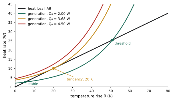
A lithium-ion cell generates heat internally, and its side reactions speed up as it warms. The cell loses heat to its surroundings in proportion to its temperature rise. If generation grows faster with temperature than the losses can, the cell can enter thermal runaway. A simple lumped model (Semenov's model of thermal explosion) for the temperature rise \(\theta\) above ambient is:

This is an autonomous first-order equation (Lesson 2). Its equilibria are where the generation curve \(Q_0e^{\beta\theta}\) meets the loss line \(hA\,\theta\). For modest \(Q_0\) they cross twice: a stable operating point and, above it, an unstable threshold. As \(Q_0\) increases, the two equilibria merge when the curve is tangent to the line, a saddle-node bifurcation. Tangency requires equal values and equal slopes: \(Q_0e^{\beta\theta} = hA\theta\) and \(\beta Q_0e^{\beta\theta} = hA\), which give \(\theta = 1/\beta\) and the critical generation:

import numpy as np
from scipy.optimize import brentq

# Cell heating: m c dT/dt = Q0 exp(beta T) - hA T, with T the rise above ambient
hA, beta = 0.5, 0.05
Q_crit = hA / (beta * np.e)
print(f"Critical heat generation {Q_crit:.2f} W, at a rise of {1 / beta:.0f} K")

for Q0 in [1.0, 2.0, 3.0, 3.5, 4.0]:
    def net(T):
        return Q0 * np.exp(beta * T) - hA * T
    T_min = np.log(hA / (Q0 * beta)) / beta
    if net(T_min) < 0:
        stable = brentq(net, 0.0, T_min)
        unstable = brentq(net, T_min, 1000.0)
        print(f"Q0 = {Q0:.1f} W: stable at +{stable:.1f} K, runaway threshold at +{unstable:.1f} K")
    else:
        print(f"Q0 = {Q0:.1f} W: no equilibrium, thermal runaway from any start")

Critical heat generation 3.68 W, at a rise of 20 K
Q0 = 1.0 W: stable at +2.2 K, runaway threshold at +71.5 K
Q0 = 2.0 W: stable at +5.2 K, runaway threshold at +50.9 K
Q0 = 3.0 W: stable at +9.8 K, runaway threshold at +35.6 K
Q0 = 3.5 W: stable at +14.3 K, runaway threshold at +27.0 K
Q0 = 4.0 W: no equilibrium, thermal runaway from any start

With the values shown, a cell generating 2 W settles 5.2 K above ambient and survives disturbances that warm it by up to about 45 K (to the threshold at 50.9 K). At 3.5 W the margin shrinks to about 13 K between the operating point and the threshold, and above 3.68 W there is no safe operating point at all. Battery engineers use more detailed versions of this analysis to size cooling (raising hA moves the critical point up), to set limits on charging current, and to design packs so that one failing cell does not heat its neighbors past their thresholds. The bifurcation picture explains why runaway can seem to come from nowhere: a small increase in load or a small loss of cooling near the critical point removes the stable state entirely.

Case study 3: how deep to bury a water main

Water mains in much of Canada are buried 2 to 3 m deep so that they do not freeze. The heat equation (Lesson 11) explains the number. Treat the ground as a deep uniform solid, with the surface temperature varying through the year as \(T_s = \bar{T} + A\cos\omega t\). A solution of \(u_t = \alpha u_{xx}\) that matches this surface condition and stays bounded at depth is:

Substituting confirms that it satisfies the heat equation: the decay and the phase shift with depth must both be governed by the same length d. The temperature swing shrinks by a factor of e for every damping depth d, and the peaks arrive later with depth, a lag of \(x/d\) radians.

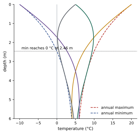
The same solution describes the daily temperature cycle in a concrete wall (with d of only about 10 to 15 cm, which is why thick walls smooth out daily swings), the skin depth of alternating current in a conductor, and the way tides penetrate into a coastal aquifer.

Common threads

The three case studies used different mathematics but the same process:

• Formulate: identify the state variables and write a balance (force, energy, mass) for each, stating every assumption.
• Simplify deliberately: a rigid building on isolators, a lumped cell, a uniform half-space. Each simplification should be one you can defend and later relax.
• Analyze before solving: find equilibria, stability, natural frequencies and time scales, since they reveal the behavior and make good checks.
• Solve by the simplest adequate method: formula, transform, series or numerical integration.
• Verify: check units, limiting cases, symmetry, a known special case or a second method.
• Interpret: translate the result into a design decision with a safety margin, and state what the model leaves out.

The course project

Choose one of the following problems, or propose your own of similar scope with your instructor's approval, and prepare a technical report with your formulation, analysis, solution (analytical where possible, numerical where necessary), verification and interpretation.

• Project A: Vehicle suspension. Model a quarter-car with a sprung and an unsprung mass (two degrees of freedom). Find its natural frequencies and modes, its frequency response to a sinusoidal road profile, and its response to a speed bump. Choose spring and damper values that balance ride comfort against road holding, and justify your choice.
• Project B: Process control. Model a tank, heater or motor as a transfer function from data or physical laws. Design P and PI controllers, find the closed-loop poles, steady-state error and step response, and determine the gain at which the loop becomes unstable. Simulate the response to a disturbance.
• Project C: Heat transfer. Analyze transient conduction in a wall, slab or fin of your choice using a Fourier series and a finite-difference model, and compare them. Use your model to answer a design question, such as the insulation thickness or fin length needed to meet a temperature limit.
• Project D: Nonlinear dynamics. Study a nonlinear system (a pendulum with forcing, a Duffing oscillator, a predator-prey or competition model with harvesting, or an electronic oscillator). Find its equilibria and their stability, draw its phase portrait numerically, identify any limit cycles or bifurcations, and explain their engineering significance.

Every report should state the governing equations and the laws they come from, list assumptions and parameter values with sources, check the solution by at least one independent means, examine sensitivity to the most uncertain parameter, and end with clear conclusions for a non-specialist reader.

Working with software

Professional practice relies on software: Python with SciPy, MATLAB and Simulink, circuit simulators, and finite element programs. Each solves differential equations numerically, and each will produce plausible-looking numbers from a wrong model or a poorly chosen tolerance. The methods of this course are what make the software trustworthy: an engineer who knows the natural frequency, time constant or equilibrium in advance can spot a wrong result immediately. A good habit is to solve a simplified version by hand first, then use software for the full problem and confirm that it reproduces the simple case.

Looking ahead

Differential equations run through the rest of an engineering program. Numerical methods (MATH-300) develop the solvers used throughout this course and analyze their accuracy and stability. Courses in vibrations, control systems, heat transfer, fluid mechanics, circuits and electromagnetics are each built on particular differential equations, and they will use transfer functions, modes, Fourier series and phase-plane ideas without stopping to re-derive them. The habits practiced here, formulating carefully, checking constantly and interpreting honestly, are the ones that matter most.