
MATH-201 · Lesson 8 of 12 · 36 min
Laplace techniques: convolution, feedback and frequency response
Lesson 7 introduced the Laplace transform and used it to solve initial value problems with steps and impulses, ending with the idea of a transfer function. This lesson builds the techniques that make the transform the everyday language of control, vibration and signal processing. It completes the partial fraction toolkit for repeated and complex poles, including the resonant case. It develops the convolution theorem, which gives the response to any input from the impulse response. It shows how transfer functions combine in block diagrams and feedback loops, and how the final value theorem predicts steady-state error. Finally, it introduces the frequency response, the Bode plot and a simple test for stability, which together let an engineer judge a system from its transfer function without solving for the time response at all.
Repeated and complex poles
Partial fractions in Lesson 7 handled distinct real poles by the cover-up rule and complex poles by completing the square. A repeated pole needs one term for each power. For a pole at \(s = a\) of multiplicity 2, the expansion contains:
The inverse of the squared term comes from the table entry \(\mathcal{L}\{te^{at}\} = 1/(s - a)^2\). The cover-up rule still gives the coefficient of the highest power; the others come from matching coefficients or substituting convenient values of s.
Worked problem
Critically damped step response
Find the unit step response of \(y'' + 2y' + y = u(t)\), starting at rest.
Show solution
- Transform: \((s^2 + 2s + 1)Y = 1/s\), so \(Y = \dfrac{1}{s(s + 1)^2}\).
- Expand: \(\dfrac{A}{s} + \dfrac{B}{s + 1} + \dfrac{C}{(s + 1)^2}\). Cover-up: \(A = 1\), \(C = 1/(-1) = -1\).
- Matching the \(s^2\) coefficient in \(1 = A(s + 1)^2 + Bs(s + 1) + Cs\): \(0 = A + B\), so \(B = -1\).
Answer: y = 1 − e^(−t) − te^(−t). It rises to 1 without overshoot, as a critically damped system should (Lesson 5).
Repeated complex poles appear in undamped resonance. The table entry needed is:
Worked problem
Resonance by Laplace transform
Solve \(x'' + 4x = \sin 2t\), \(x(0) = x'(0) = 0\).
Show solution
- Transform: \((s^2 + 4)X = \dfrac{2}{s^2 + 4}\), so \(X = \dfrac{2}{(s^2 + 4)^2}\).
- With \(\omega = 2\), \(2\omega^3 = 16\), so \(X = \tfrac{1}{8}\cdot\dfrac{16}{(s^2 + 4)^2}\).
Answer: x = (1/8)(sin 2t − 2t cos 2t). The t cos 2t term grows without bound: forcing at the natural frequency with no damping gives an amplitude that increases linearly, about t/4. The double pole on the imaginary axis is the s-domain signature of resonance.
The convolution theorem
Lesson 7 mentioned that a product in the s-domain corresponds to a convolution in time. Stated fully: if \(F(s) = \mathcal{L}\{f\}\) and \(G(s) = \mathcal{L}\{g\}\), then
Since the output of a system at rest is \(Y = GF\), and \(g(t)\), the inverse of G, is the impulse response, the response to any input is the convolution of the input with the impulse response. This is Duhamel's integral from Lesson 4, now valid for any linear system: measure a system's impulse response once (for example with a hammer test), and its response to any other input can be computed. Convolution is also a quick way to invert some products directly.
Worked problem
Inverting by convolution
Find \(\mathcal{L}^{-1}\left\{\dfrac{1}{s(s^2 + 1)}\right\}\).
Show solution
- Write it as \(\dfrac{1}{s}\cdot\dfrac{1}{s^2 + 1}\), the transforms of 1 and \(\sin t\).
- Convolve: \(\int_0^t \sin\tau \cdot 1\,d\tau = 1 - \cos t\).
Answer: 1 − cos t, the response of an undamped oscillator to a unit step: it oscillates about the new static position, reaching twice the static deflection.
Worked problem
Sensor lag
A temperature probe behaves as a first-order system with time constant τ = 10 s: \(\tau y' + y = f(t)\). The true temperature rises steadily, \(f = rt\) with r = 0.5 °C/s. Find the reading, and the error once the transient has died away.
Show solution
- The impulse response is \(g(t) = \tfrac{1}{\tau}e^{-t/\tau}\).
- Convolve, using \(\sigma\) as the integration variable: \(y = \int_0^t r\sigma\,\tfrac{1}{\tau}e^{-(t - \sigma)/\tau}\,d\sigma = r\left(t - \tau + \tau e^{-t/\tau}\right)\).
- After a few time constants, \(y \approx r(t - \tau)\): the reading follows the true value delayed by τ.
Answer: The probe lags by τ = 10 s, so it reads 0.5 × 10 = 5 °C low throughout the ramp. Engineers choose sensors whose time constants are short compared with the process they measure, or correct for the known lag.
Block diagrams and feedback
Transfer functions make it easy to combine components. Two systems in series multiply: \(G_1G_2\). Two in parallel add: \(G_1 + G_2\). The most important combination is the feedback loop, in which a controller C(s) compares the measured output with a set point R(s) and drives the process G(s) with the error. With unity feedback, \(E = R - Y\) and \(Y = CGE\), so:
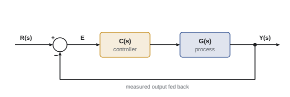
The denominator \(1 + CG\) sets the closed-loop poles, so feedback changes the speed and stability of a system, not just its gain. The final value theorem (Lesson 7) predicts the steady-state error for a step in the set point.
Worked problem
Proportional and PI control of a tank heater
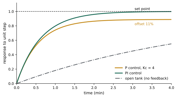
A heater and tank have \(G(s) = \dfrac{2}{5s + 1}\) (gain 2 °C per unit of heater signal, time constant 5 min). Compare a proportional controller \(C = K_c = 4\) with a PI controller \(C = 4\left(1 + \dfrac{1}{5s}\right)\) for a unit step in the set point.
Show solution
- P control: \(CG = \dfrac{8}{5s + 1}\), so \(\dfrac{Y}{R} = \dfrac{8}{5s + 9}\). Final value for \(R = 1/s\): \(8/9 = 0.889\). Closed-loop time constant \(5/9 = 0.56\) min.
- PI control: \(C = \dfrac{4(5s + 1)}{5s}\), so \(CG = \dfrac{8}{5s}\) (the controller zero cancels the process pole) and \(\dfrac{Y}{R} = \dfrac{8}{5s + 8}\).
- Final value: \(8/8 = 1\). Time constant \(5/8 = 0.63\) min.
Answer: Feedback makes both loops eight to nine times faster than the open tank. Proportional control leaves an 11% offset; the integral term removes it entirely, because any remaining error would keep the integral growing. This is why PI control is the industrial default.
Frequency response and Bode plots
When a stable linear system is driven by a sinusoid \(\sin\omega t\), the transient dies away and the output becomes a sinusoid at the same frequency, scaled and shifted:
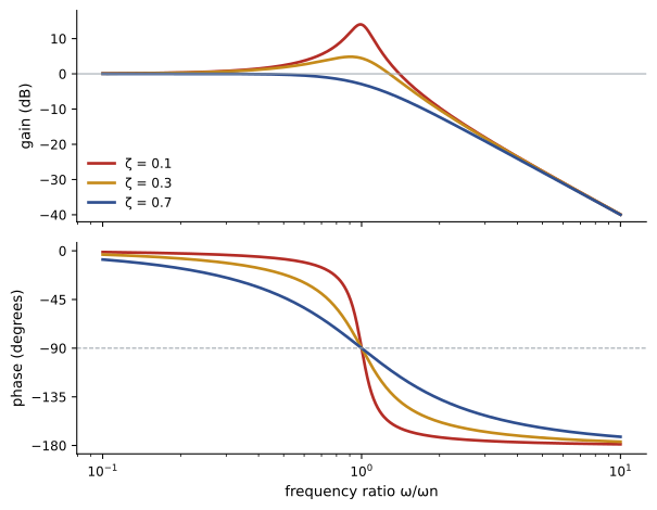
So the frequency response is just the transfer function evaluated at \(s = i\omega\): its magnitude is the gain and its angle is the phase shift. A Bode plot shows both against frequency on logarithmic axes, with the gain in decibels, \(20\log_{10}|G|\). Engineers use Bode plots to design filters, specify sensors and amplifiers, and assess the stability margins of control loops.
For a first-order system \(G = 1/(\tau s + 1)\), the gain is \(1/\sqrt{1 + \omega^2\tau^2}\) and the phase is \(-\arctan\omega\tau\). At the corner frequency \(\omega = 1/\tau\), the gain is \(1/\sqrt{2}\) (−3 dB) and the phase is −45°; above it, the gain falls by 20 dB for every tenfold increase in frequency.
Worked problem
An RC low-pass filter
An RC filter with R = 1 kΩ and C = 1 µF has \(G = 1/(RCs + 1)\). Find the corner frequency in hertz and the gain and phase at 1 kHz.
Show solution
- \(\tau = RC = 10^{-3}\) s, so the corner is 1000 rad/s, or 159 Hz.
- At 1 kHz, \(\omega\tau = 2\pi \times 1000 \times 10^{-3} = 6.28\).
- Gain: \(1/\sqrt{1 + 6.28^2} = 0.157\), or −16 dB. Phase: \(-\arctan 6.28 = -81°\).
Answer: Corner 159 Hz; at 1 kHz the signal is reduced to 16% (−16 dB) and lags by 81°. Signals well below 159 Hz pass almost unchanged, so the filter removes high-frequency noise from a slowly varying measurement.
For the second-order system \(G = \omega_n^2/(s^2 + 2\zeta\omega_ns + \omega_n^2)\), the gain is the amplification factor of Lesson 5. A lightly damped system shows a sharp resonant peak of height about \(1/(2\zeta)\) near \(\omega_n\), and the phase swings through −90° at \(\omega_n\) toward −180°.
Stability from the transfer function
A linear system is stable if every pole of its transfer function has a negative real part, so that every mode decays. For a closed loop, the poles are the roots of \(1 + CG = 0\). For low-order polynomials there are simple tests that avoid finding the roots. A second-order polynomial \(s^2 + a_1s + a_0\) has both roots in the left half-plane exactly when \(a_1 > 0\) and \(a_0 > 0\). For a cubic \(s^3 + a_2s^2 + a_1s + a_0\), the Routh-Hurwitz criterion requires all coefficients positive and
Worked problem
How much gain is too much?
A process made of three identical lags, \(G = \dfrac{1}{(s + 1)^3}\), is controlled with a proportional gain K and unity feedback. For what K is the loop stable?
Show solution
- Characteristic equation: \((s + 1)^3 + K = s^3 + 3s^2 + 3s + 1 + K = 0\).
- Routh-Hurwitz: \(3 \times 3 > 1 + K\), so \(K < 8\).
- At K = 8, the polynomial factors as \((s + 3)(s^2 + 3)\): poles at \(\pm i\sqrt{3}\), a sustained oscillation at 1.73 rad/s.
Answer: Stable for 0 < K < 8. Raising the gain speeds up the response and reduces offset, but past K = 8 the loop oscillates with growing amplitude. Every real control loop faces this trade-off, and the Bode plot measures how far a design is from the edge (its gain and phase margins).
import numpy as np

# Process G = 1/(s + 1)^3 with proportional gain K and unity feedback
# Closed-loop characteristic polynomial: s^3 + 3s^2 + 3s + (1 + K)
for K in [2, 6, 8, 10]:
    poles = np.roots([1, 3, 3, 1 + K])
    worst = max(poles.real)
    if worst < -1e-6:
        status = "stable"
    elif worst < 1e-6:
        status = "on the edge"
    else:
        status = "unstable"
    p = sorted(poles, key=lambda z: z.real)
    text = ", ".join(f"{round(z.real, 3) + 0.0:.3f}{z.imag:+.3f}j" for z in p)
print(f"K = {K:2d}: poles {text} ({status})")K = 2: poles -2.260+0.000j, -0.370+1.091j, -0.370-1.091j (stable) K = 6: poles -2.817+0.000j, -0.091+1.574j, -0.091-1.574j (stable) K = 8: poles -3.000+0.000j, 0.000+1.732j, 0.000-1.732j (on the edge) K = 10: poles -3.154+0.000j, 0.077+1.866j, 0.077-1.866j (unstable)
Common mistakes
MistakeWriting only one term for a repeated pole.
InsteadA pole of multiplicity m needs m terms, one for each power.
MistakeTreating L⁻¹{FG} as the product of the inverses.
InsteadA product of transforms inverts to a convolution, not a product.
MistakeForgetting the minus sign in the feedback formula.
InsteadWith negative feedback, Y/R = CG/(1 + CG).
MistakeApplying the frequency response to an unstable system.
InsteadA steady sinusoidal response exists only when all poles are in the left half-plane.
MistakeAssuming more controller gain always helps.
InsteadHigh gain can destabilize the loop; check the closed-loop poles.
Summary and key terms
- Repeated poles give terms te^(at); double imaginary poles give resonance, t cos ωt.
- The convolution theorem: L⁻¹{FG} = ∫₀ᵗ f(τ)g(t − τ) dτ; the response is input convolved with impulse response.
- A first-order sensor follows a ramp with a lag equal to its time constant.
- Series blocks multiply, and unity feedback gives Y/R = CG/(1 + CG).
- Proportional control leaves a steady-state offset; integral action removes it.
- The frequency response is G(iω): gain |G| and phase ∠G, plotted on a Bode plot.
- Stability requires all poles in the left half-plane; Routh-Hurwitz tests this for low-order polynomials.
- Repeated pole
- A root of the denominator that occurs more than once.
- Convolution
- The integral ∫₀ᵗ f(τ)g(t − τ) dτ, whose transform is F(s)G(s).
- Block diagram
- A diagram of connected transfer functions.
- Feedback loop
- A system in which the measured output is compared with a set point to drive the input.
- Steady-state error
- The difference between set point and output after transients die away.
- PI controller
- A controller with proportional and integral terms.
- Frequency response
- The gain and phase of a system's steady response to sinusoids, G(iω).
- Bode plot
- Gain in decibels and phase plotted against frequency on logarithmic axes.
- Corner frequency
- The frequency 1/τ where a first-order system's gain is down 3 dB.
- Routh-Hurwitz criterion
- Conditions on polynomial coefficients that guarantee all roots have negative real parts.
Practice problems
Work each problem on paper first, then reveal the answer to check.
Find \(\mathcal{L}^{-1}\left\{\dfrac{1}{(s + 2)^2}\right\}\).
Show answer
te^(−2t).
Find \(\mathcal{L}^{-1}\left\{\dfrac{s + 3}{(s + 1)^2}\right\}\).
Show answer
(s + 1 + 2)/(s + 1)²: e^(−t) + 2te^(−t).
Use convolution to find \(\mathcal{L}^{-1}\left\{\dfrac{1}{s(s + a)}\right\}\).
Show answer
∫₀ᵗ e^(−aτ) dτ = (1 − e^(−at))/a.
A probe with τ = 4 s measures a temperature rising at 2 °C/min. What is the steady lag error?
Show answer
rτ = (2/60) × 4 = 0.13 °C.
Find the closed-loop transfer function for C = 10 and G = 1/(s + 2) with unity feedback.
Show answer
10/(s + 12).
In that loop, what is the steady-state error for a unit step?
Show answer
Output 10/12 = 0.833; error 0.167.
Find the gain in decibels of G = 1/(0.1s + 1) at ω = 100 rad/s.
Show answer
1/√101 ≈ 0.0995, about −20 dB.
What is the phase of G = 1/(τs + 1) at its corner frequency?
Show answer
−45°.
Is \(s^3 + 2s^2 + 3s + 7\) stable?
Show answer
No: 2 × 3 = 6 < 7.
For G = K/((s + 1)(s + 2)(s + 3)) with unity feedback, find the largest stable K.
Show answer
s³ + 6s² + 11s + 6 + K: 66 > 6 + K, so K < 60.
Lesson quiz · 5 questions
Score 60% or more to complete this lesson.
Create a free account to save your progress, take quizzes and earn a certificate.