
MATH-209 · Lesson 2 of 12 · 33 min
Vector functions, curves and motion
Lesson 1 described quantities that vary over a region, such as temperature over a plate. Many engineering problems instead follow something along a path: a vehicle on a highway, the tip of a robot arm, a satellite in orbit, a cutting tool on a machining center, the centerline of a pipe or a cable. The natural description is a vector function, which gives a position vector for each value of a parameter, usually time. This lesson develops the calculus of vector functions. Derivatives give velocity and acceleration; integrals recover position from acceleration; arc length and curvature describe the geometry of the path itself; and splitting acceleration into tangential and normal parts, or into radial and transverse parts, explains the forces felt by a driver on a curve or a part moving along a rotating arm. The ideas reappear in Lesson 7, where integrals along curves are used to compute work and circulation.
Vector functions and space curves
A vector function assigns a vector to each value of a parameter t:
As t varies, the tip of \(\mathbf{r}(t)\) traces a curve in space. The same curve can be traced by different parametrizations, quickly or slowly, forward or backward; the parametrization carries the information about motion, while the curve itself is only the path. Two standard examples:
- A straight line through \(\mathbf{r}_0\) in direction \(\mathbf{v}\): \(\mathbf{r}(t) = \mathbf{r}_0 + t\mathbf{v}\) (MATH-125).
- A circular helix of radius a that rises \(2\pi b\) per turn: \(\mathbf{r}(t) = a\cos t\,\mathbf{i} + a\sin t\,\mathbf{j} + bt\,\mathbf{k}\). Helices describe coil springs, spiral ramps, screw threads, DNA and the path of a charged particle in a magnetic field.
Limits, continuity and derivatives of vector functions are taken component by component.
Velocity, speed and acceleration
If \(\mathbf{r}(t)\) is the position of a particle, its velocity and acceleration are
The velocity vector is tangent to the path and points in the direction of motion; its length is the speed. The unit tangent vector is \(\mathbf{T} = \mathbf{v}/|\mathbf{v}|\). Going the other way, integrating the acceleration twice, with the initial velocity and position as constants of integration, recovers the motion. This is how inertial navigation systems in aircraft and phones estimate position from accelerometer readings, and why small sensor errors make the position estimate drift: an error in acceleration is integrated twice.
Worked problem
A projectile
A ball is launched from the origin at 20 m/s and 30° above the horizontal. Ignoring air resistance, find its position, its maximum height and its range.
Show solution
- Acceleration: \(\mathbf{a} = -9.81\,\mathbf{j}\). Initial velocity: \(\mathbf{v}(0) = 20\cos 30°\,\mathbf{i} + 20\sin 30°\,\mathbf{j} = 17.32\,\mathbf{i} + 10\,\mathbf{j}\).
- Integrate: \(\mathbf{v}(t) = 17.32\,\mathbf{i} + (10 - 9.81t)\,\mathbf{j}\), then \(\mathbf{r}(t) = 17.32t\,\mathbf{i} + (10t - 4.905t^2)\,\mathbf{j}\).
- Maximum height when the vertical velocity is zero, \(t = 1.019\) s: \(y = 5.10\) m.
- Landing when \(y = 0\): \(t = 2.039\) s, so the range is \(17.32 \times 2.039 = 35.3\) m.
Answer: r(t) = 17.32t i + (10t − 4.905t²) j, with maximum height 5.10 m and range 35.3 m. The calculation is a vector version of the integration in MATH-100; with air resistance the acceleration depends on velocity and a numerical solution is needed (MATH-201).
Arc length
The distance traveled along the curve from \(t = a\) to \(t = b\) is the integral of the speed:
This extends the arc length formula of MATH-101 to curves in space. Measuring position by arc length s instead of time gives the arc length parametrization, in which the curve is traced at unit speed. Road and rail alignments, pipe routes and tool paths are specified this way, by chainage (distance along the centerline).
Worked problem
A parking-garage ramp
A spiral ramp has a centerline radius of 15 m and rises 3.0 m per full turn. Find the length of the centerline per turn and the average grade.
Show solution
- Helix with \(a = 15\) and \(2\pi b = 3.0\), so \(b = 0.477\) m.
- Speed in the parameter: \(|\mathbf{r}'| = \sqrt{a^2\sin^2 t + a^2\cos^2 t + b^2} = \sqrt{a^2 + b^2} = 15.008\).
- Length per turn: \(2\pi \times 15.008 = 94.3\) m. Grade: \(3.0/94.3 = 3.2\%\).
Answer: About 94.3 m per turn, at a grade of 3.2%. The helix is barely longer than the circle beneath it (94.2 m), because the rise is small compared with the circumference.
Curvature
Curvature measures how sharply a curve bends: how fast the unit tangent turns per unit distance traveled. For a circle of radius R it is \(1/R\), and for a straight line it is zero. In general, the radius of curvature \(\rho = 1/\kappa\) is the radius of the circle that best fits the curve at that point. A convenient formula, valid for any parametrization, is
For a plane curve \(y = f(x)\), this reduces to \(\kappa = |f''|/(1 + f'^2)^{3/2}\), which for small slopes is approximately \(|f''|\), the approximation used in beam theory, where the curvature of the deflected beam is \(M/(EI)\).
Worked problem
Curvature of a helix
Find the curvature of the helix \(\mathbf{r} = a\cos t\,\mathbf{i} + a\sin t\,\mathbf{j} + bt\,\mathbf{k}\), and apply it to the ramp.
Show solution
- \(\mathbf{r}' = (-a\sin t, a\cos t, b)\) and \(\mathbf{r}'' = (-a\cos t, -a\sin t, 0)\).
- \(\mathbf{r}' \times \mathbf{r}'' = (ab\sin t, -ab\cos t, a^2)\), with magnitude \(a\sqrt{a^2 + b^2}\).
- \(\kappa = \dfrac{a\sqrt{a^2 + b^2}}{(a^2 + b^2)^{3/2}} = \dfrac{a}{a^2 + b^2}\).
- Ramp: \(\kappa = 15/(225 + 0.228) = 0.0666\) m⁻¹, a radius of curvature of 15.02 m.
Answer: κ = a/(a² + b²), constant along the helix. For the ramp the radius of curvature is essentially the plan radius, so a driver steers as if on a flat circle.
Transition curves
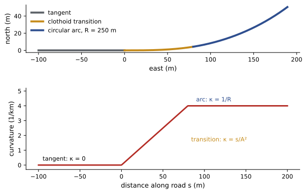
A road or railway cannot jump straight from a tangent (zero curvature) to a circular arc (constant curvature): the sideways acceleration would change suddenly, jolting passengers and loads. Designers insert a transition curve, usually a clothoid (Euler spiral), whose curvature increases in proportion to arc length, \(\kappa = s/A^2\). The lateral acceleration then builds up at a steady rate as the vehicle enters the curve. The same idea, limiting the rate of change of acceleration (the jerk), shapes elevator motion profiles, cam designs and robot trajectories.
Tangential and normal acceleration
Acceleration can be split into a part along the path, which changes the speed, and a part perpendicular to it, toward the center of curvature, which changes the direction:
Here \(\mathbf{N}\) is the unit normal, pointing toward the center of curvature. The normal (centripetal) acceleration grows with the square of speed and with curvature, which is why speed limits drop sharply on tight curves. Together with the binormal \(\mathbf{B} = \mathbf{T} \times \mathbf{N}\), the vectors T and N form a moving frame (the Frenet frame) that travels with the particle; the rate at which B turns, the torsion, measures how the curve twists out of a plane.
Worked problem
A highway curve
A car travels at 100 km/h around a curve of radius 250 m while braking at 2.0 m/s². Find the normal and total acceleration.
Show solution
- \(v = 100/3.6 = 27.8\) m/s, so \(a_N = 27.8^2/250 = 3.09\) m/s².
- \(a_T = -2.0\) m/s² (braking).
- Total: \(\sqrt{3.09^2 + 2.0^2} = 3.68\) m/s², or 0.38g.
Answer: The car needs 3.68 m/s² of total grip, 0.38 of its weight. Tire friction must supply this, so braking hard in a curve uses up grip that would otherwise be available for cornering. Highway design guides combine this calculation with superelevation (banking) to set minimum curve radii for each design speed.
Motion in polar coordinates
For motion in a plane described by distance r and angle θ, as for a part sliding along a rotating arm or a satellite in orbit, it is natural to use the unit vectors \(\mathbf{e}_r\) (outward) and \(\mathbf{e}_\theta\) (perpendicular, in the direction of increasing θ). Since these vectors turn as θ changes, differentiating \(\mathbf{r} = r\,\mathbf{e}_r\) twice gives
The term \(-r\dot{\theta}^2\) is the centripetal acceleration and \(2\dot{r}\dot{\theta}\) is the Coriolis acceleration, which appears whenever something moves radially on a rotating body.
Worked problem
A robot arm
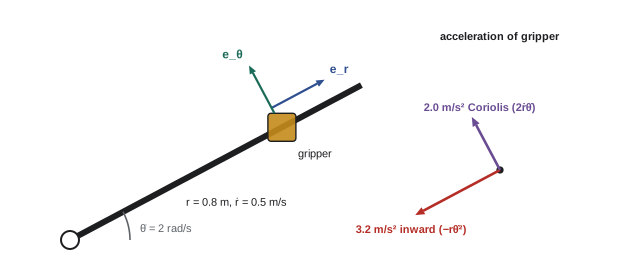
A gripper slides outward along a robot arm at a constant 0.5 m/s while the arm rotates at a constant 2.0 rad/s. Find the gripper's acceleration when it is 0.8 m from the axis.
Show solution
- \(\dot{r} = 0.5\), \(\ddot{r} = 0\), \(\dot{\theta} = 2.0\), \(\ddot{\theta} = 0\), \(r = 0.8\).
- Radial: \(0 - 0.8 \times 2.0^2 = -3.2\) m/s² (toward the axis).
- Transverse: \(0 + 2 \times 0.5 \times 2.0 = 2.0\) m/s².
Answer: The acceleration is 3.2 m/s² inward and 2.0 m/s² sideways, 3.77 m/s² in total. The sideways Coriolis part must be supplied by the arm pushing on the gripper, a load that a designer considering only the centripetal term would miss.
Circular orbits
For a satellite in a circular orbit of radius r, gravity supplies exactly the normal acceleration: \(v^2/r = GM/r^2\), where \(GM = 3.986 \times 10^{14}\) m³/s² for the Earth. So the orbital speed is \(v = \sqrt{GM/r}\) and the period is \(T = 2\pi r/v = 2\pi\sqrt{r^3/GM}\). At 400 km altitude (r = 6771 km), this gives v = 7.67 km/s and a period of 92.4 minutes, the orbit of the International Space Station. Setting T equal to one sidereal day (86 164 s) gives r = 42 164 km, the geostationary orbit used by communication and weather satellites, which appear fixed in the sky. Here the acceleration is entirely normal: the speed is constant and the satellite falls continuously toward the Earth while moving sideways fast enough to keep missing it. The same balance sets the speed of a vehicle on a banked curve with no reliance on friction, and the magnetic field strength needed to bend a particle beam into a circle in an accelerator.
Common mistakes
MistakeConfusing the curve with its parametrization.
InsteadThe curve is the path; the parametrization adds speed and direction of travel.
MistakeComputing arc length as ∫ r(t) dt.
InsteadArc length integrates the speed |r′(t)|.
MistakeUsing |r″| as the curvature for a general parametrization.
InsteadUse κ = |r′ × r″|/|r′|³; |r″| works only at unit speed.
MistakeForgetting the tangential part of acceleration when the speed changes.
InsteadTotal acceleration combines a_T = d|v|/dt and a_N = v²/ρ.
MistakeOmitting the Coriolis term for radial motion on a rotating body.
InsteadThe transverse acceleration is rθ̈ + 2ṙθ̇.
Summary and key terms
- A vector function r(t) traces a curve; derivatives are taken component by component.
- Velocity r′ is tangent to the path, speed is |r′| and acceleration is r″.
- Integrating acceleration with initial conditions recovers velocity and position.
- Arc length is the integral of speed.
- Curvature κ = |r′ × r″|/|r′|³; a helix has κ = a/(a² + b²).
- Acceleration splits into a_T = d|v|/dt along the path and a_N = κv² toward the center of curvature.
- In polar coordinates, a = (r̈ − rθ̇²) e_r + (rθ̈ + 2ṙθ̇) e_θ, including the Coriolis term.
- Vector function
- A function that assigns a vector to each value of a parameter.
- Helix
- A curve winding around a cylinder at a constant rate of rise.
- Unit tangent vector
- T = v/|v|, the direction of motion.
- Arc length
- Distance measured along a curve.
- Curvature
- The rate at which the unit tangent turns per unit arc length.
- Radius of curvature
- The radius 1/κ of the best-fitting circle.
- Clothoid
- A transition curve whose curvature is proportional to arc length.
- Normal acceleration
- The component of acceleration toward the center of curvature, v²/ρ.
- Frenet frame
- The moving frame of unit tangent, normal and binormal vectors.
- Coriolis acceleration
- The term 2ṙθ̇ arising from radial motion on a rotating body.
Practice problems
Work each problem on paper first, then reveal the answer to check.
Find the velocity and speed of \(\mathbf{r}(t) = (t^2, 2t, 3)\) at t = 1.
Show answer
v = (2, 2, 0); speed 2√2.
A particle has \(\mathbf{a} = (0, 0, -9.81)\), \(\mathbf{v}(0) = (3, 4, 10)\) and \(\mathbf{r}(0) = \mathbf{0}\). Find \(\mathbf{r}(t)\).
Show answer
(3t, 4t, 10t − 4.905t²).
Find the length of \(\mathbf{r}(t) = (3\cos t, 3\sin t, 4t)\) for 0 ≤ t ≤ 2π.
Show answer
|r′| = 5, so L = 10π ≈ 31.4.
Find the curvature of that helix.
Show answer
κ = 3/(9 + 16) = 0.12.
Find the curvature of \(y = x^2\) at x = 0 and at x = 1.
Show answer
2 at x = 0; 2/5^(3/2) = 0.179 at x = 1.
A train at 30 m/s rounds a curve of radius 600 m. Find its normal acceleration.
Show answer
900/600 = 1.5 m/s².
What curve radius limits normal acceleration to 1.0 m/s² at 80 km/h?
Show answer
v = 22.2 m/s; ρ = 494 m.
A car speeds up at 1.5 m/s² while at 20 m/s on a 200 m radius curve. Total acceleration?
Show answer
a_N = 2.0, a_T = 1.5: total 2.5 m/s².
A bead slides out along a rod rotating at 3 rad/s with ṙ = 0.2 m/s. Find the Coriolis acceleration.
Show answer
2 × 0.2 × 3 = 1.2 m/s².
Why does an inertial navigation position estimate drift?
Show answer
Acceleration errors are integrated twice, so position error grows rapidly with time.
Lesson quiz · 5 questions
Score 60% or more to complete this lesson.
Create a free account to save your progress, take quizzes and earn a certificate.