
MATH-209 · Lesson 4 of 12 · 37 min
Optimization in several variables
Lesson 3 introduced critical points, the second derivative test and Lagrange multipliers. Optimization is so central to engineering that it deserves a closer look. Designers minimize weight, cost, energy use and error, and maximize strength, efficiency and output, almost always with several variables and several constraints. This lesson strengthens the theory and widens the toolkit. It explains the second derivative test through the second-order Taylor expansion and the Hessian matrix, which extends naturally to three or more variables; finds absolute extremes on closed regions; derives the method of least squares as an optimization problem; looks more deeply at Lagrange multipliers, including what the multiplier means and how to handle two constraints and inequality constraints; and finishes with the numerical methods, gradient descent and Newton's method, that solve the large problems found in practice.
The Hessian and the second derivative test
Near a point \(\mathbf{a}\), a smooth function of several variables is approximated by its second-order Taylor expansion. Writing \(\mathbf{h}\) for the small displacement from \(\mathbf{a}\):
Here H is the Hessian matrix of second partial derivatives, which is symmetric because mixed partial derivatives are equal:
At a critical point the gradient term vanishes, so the behavior is set by the quadratic form \(\mathbf{h}^TH\mathbf{h}\) (MATH-125). If it is positive for every direction, the point is a local minimum; if negative for every direction, a local maximum; if positive in some directions and negative in others, a saddle. Since a symmetric matrix can be diagonalized by rotating the axes, the test reduces to the signs of the eigenvalues of H:
- All eigenvalues positive (H positive definite): local minimum.
- All eigenvalues negative: local maximum.
- Eigenvalues of both signs: saddle point.
- Some eigenvalue zero: the test is inconclusive.
In two variables, the determinant \(D = f_{xx}f_{yy} - f_{xy}^2\) is the product of the two eigenvalues, which is why the test in Lesson 3 works: D > 0 means the eigenvalues share a sign, and \(f_{xx}\) tells which. The eigenvectors give the principal directions of curvature, the directions in which the surface curves most and least.
Worked problem
A minimum in three variables
Find and classify the critical point of \(f = 2x^2 + y^2 + 3z^2 + 2xy - 4x - 2y\).
Show solution
- Gradient: \(f_x = 4x + 2y - 4\), \(f_y = 2x + 2y - 2\), \(f_z = 6z\). Setting all to zero gives \(x = 1\), \(y = 0\), \(z = 0\).
- \[H = \begin{pmatrix} 4 & 2 & 0 \\ 2 & 2 & 0 \\ 0 & 0 & 6 \end{pmatrix}\]
- Eigenvalues: 6, and those of \(\begin{pmatrix} 4 & 2 \\ 2 & 2 \end{pmatrix}\), which are \(3 \pm \sqrt{5}\), or 5.24 and 0.76.
Answer: All eigenvalues are positive, so (1, 0, 0) is a minimum, with f = −2. The small eigenvalue 0.76 shows that the bowl is shallow in one direction, a fact that matters for numerical methods later in this lesson.
Absolute extremes on a closed region
A continuous function on a closed, bounded region always attains an absolute maximum and minimum. To find them: locate the critical points inside the region, find the extremes on the boundary (by parametrizing it, or with Lagrange multipliers), and compare all the candidate values.
Worked problem
Hot and cold spots on a disc
The temperature on a circular plate \(x^2 + y^2 \le 1\) is \(T = x^2 + 2y^2 - x\) (in units of 10 °C above ambient). Find the hottest and coldest points.
Show solution
- Interior: \(T_x = 2x - 1 = 0\), \(T_y = 4y = 0\), giving \((\tfrac{1}{2}, 0)\) with \(T = -\tfrac{1}{4}\).
- Boundary: with \(x = \cos\theta\), \(y = \sin\theta\), \(T = \cos^2\theta + 2\sin^2\theta - \cos\theta = 2 - \cos^2\theta - \cos\theta\).
- With \(u = \cos\theta\) in \([-1, 1]\), \(T = 2 - u - u^2\), whose maximum is at \(u = -\tfrac{1}{2}\): \(T = 2.25\) at \((-\tfrac{1}{2}, \pm\tfrac{\sqrt{3}}{2})\). At \(u = 1\), \(T = 0\).
Answer: Coldest: (½, 0), at T = −0.25 (2.5 °C below ambient). Hottest: (−½, ±√3/2) on the rim, at T = 2.25 (22.5 °C above ambient). The maximum lies on the boundary, which a search for interior critical points alone would have missed.
Least squares as optimization
When a model \(y = mx + c\) is fitted to measured points \((x_i, y_i)\), the best fit in the least-squares sense minimizes the sum of squared errors:
Setting \(\partial E/\partial m = 0\) and \(\partial E/\partial c = 0\) gives the normal equations:
These are the same normal equations that MATH-125 derives geometrically by projection. The Hessian of E has positive eigenvalues whenever the \(x_i\) are not all equal, so the critical point is the minimum.
Worked problem
Fitting a calibration line
Fit a line to the points (0, 1), (1, 3), (2, 4), (3, 4).
Show solution
- Sums: \(\sum x = 6\), \(\sum x^2 = 14\), \(\sum y = 12\), \(\sum xy = 23\), n = 4.
- Normal equations: \(14m + 6c = 23\) and \(6m + 4c = 12\).
- From the second, \(c = 3 - 1.5m\); substituting, \(5m = 5\), so \(m = 1\) and \(c = 1.5\).
Answer: y = x + 1.5. The residuals are −0.5, 0.5, 0.5 and −0.5, summing to zero, as they always do for a least-squares line with an intercept.
Lagrange multipliers revisited
What the multiplier means
In the method \(\nabla f = \lambda\nabla g\) with constraint \(g = c\), the multiplier is not just an auxiliary unknown. If \(f^*(c)\) is the optimal value, then
So \(\lambda\) is the rate at which the best achievable objective changes as the constraint is relaxed. Economists call it a shadow price; for an engineer it answers questions such as "how much more material does each extra liter of capacity cost?" without re-solving the problem.
Worked problem
The minimum-material can
A closed cylindrical can must hold V = 1000 cm³. Find the radius and height that minimize the surface area, and interpret the multiplier.
Show solution
- Minimize \(A = 2\pi r^2 + 2\pi rh\) subject to \(\pi r^2h = V\).
- Lagrange: \(4\pi r + 2\pi h = \lambda\,2\pi rh\) and \(2\pi r = \lambda\pi r^2\). The second gives \(\lambda = 2/r\); substituting into the first, \(2r + h = 2h\), so \(h = 2r\).
- Then \(2\pi r^3 = 1000\): \(r = 5.42\) cm, \(h = 10.84\) cm, \(A = 6\pi r^2 = 554\) cm².
- \(\lambda = 2/r = 0.369\) cm² per cm³.
Answer: r = 5.42 cm and h = 10.84 cm: the height equals the diameter. Each extra cubic centimeter of capacity costs about 0.37 cm² of material, so a 1.1 L can would need about 37 cm² more. Real cans are taller than this optimum because the ends are thicker and more expensive to form than the sides, which changes the objective.
Worked problem
Cutting a beam from a log
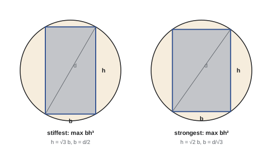
A rectangular beam of width b and depth h is cut from a log of diameter d, so \(b^2 + h^2 = d^2\). Bending stiffness is proportional to \(bh^3\) and bending strength to \(bh^2\). Find the best proportions for each.
Show solution
- Stiffness: \(\nabla(bh^3) = \lambda\nabla(b^2 + h^2)\) gives \(h^3 = 2\lambda b\) and \(3bh^2 = 2\lambda h\). Dividing, \(h^2 = 3b^2\), so \(h = \sqrt{3}\,b\), with \(b = d/2\).
- Strength: \(\nabla(bh^2) = \lambda\nabla(b^2 + h^2)\) gives \(h^2 = 2\lambda b\) and \(2bh = 2\lambda h\), so \(h^2 = 2b^2\), \(h = \sqrt{2}\,b\), with \(b = d/\sqrt{3}\).
- For d = 400 mm: stiffest beam 200 × 346 mm; strongest beam 231 × 327 mm.
Answer: Depth-to-width ratios of √3 ≈ 1.73 for stiffness and √2 ≈ 1.41 for strength. Different objectives give different optima from the same constraint, so the design goal must be decided before optimizing.
Two constraints
With two constraints \(g = c_1\) and \(h = c_2\), the feasible set is usually a curve, and at the optimum the gradient of f lies in the plane spanned by the two constraint gradients:
Worked problem
Highest point on an elliptical cut
The plane \(x + y + z = 1\) cuts the cylinder \(x^2 + y^2 = 1\) in an ellipse. Find its highest and lowest points.
Show solution
- Optimize \(f = z\): \((0, 0, 1) = \lambda(1, 1, 1) + \mu(2x, 2y, 0)\).
- The third component gives \(\lambda = 1\); then \(1 + 2\mu x = 0\) and \(1 + 2\mu y = 0\), so \(x = y\).
- With \(x^2 + y^2 = 1\): \(x = y = \pm 1/\sqrt{2}\), and \(z = 1 - x - y = 1 \mp \sqrt{2}\).
Answer: Highest point (−1/√2, −1/√2, 1 + √2) and lowest point (1/√2, 1/√2, 1 − √2).
Inequality constraints
Real constraints are usually inequalities: stress must not exceed the allowable value, a budget must not be overspent. At the optimum, each inequality is either inactive (not binding, so it can be ignored locally) or active (holding with equality, so it acts like an equality constraint with a multiplier of the correct sign). These are the Karush-Kuhn-Tucker (KKT) conditions, the basis of the optimization software used for structural design and operations planning. In practice, one tries the cases: solve with no constraints active, check feasibility, then make constraints active one at a time.
Worked problem
A budget constraint
Maximize the output \(f = xy\) of a process that uses x units of one resource at cost 1 and y units of another at cost 2, with a budget \(x + 2y \le 10\) and \(x, y \ge 0\).
Show solution
- With the budget inactive, f has no interior maximum (it grows without limit), so the budget must be active.
- Lagrange on \(x + 2y = 10\): \(y = \lambda\), \(x = 2\lambda\), so \(4\lambda = 10\), \(\lambda = 2.5\).
Answer: x = 5, y = 2.5, giving f = 12.5. The multiplier 2.5 says one more unit of budget would raise the output by about 2.5, and it is positive, as it must be for an active "less than or equal" constraint in a maximization.
Numerical optimization
Most engineering optimization problems have too many variables, or functions too complex, for these hand methods. Numerical methods search iteratively. Gradient descent steps repeatedly in the direction of steepest descent, \(-\nabla f\) (Lesson 3), with a step size \(\alpha\):
It is simple and needs only the gradient, but it is slow when the bowl is long and narrow, that is, when the eigenvalues of the Hessian differ greatly: the steps zigzag across the valley. Newton's method uses the Hessian as well, jumping to the minimum of the local quadratic model, \(\mathbf{x}_{k+1} = \mathbf{x}_k - H^{-1}\nabla f\), and converges in very few steps near the optimum, at the cost of computing and solving with H. Practical software uses compromises (quasi-Newton methods such as BFGS) that build up an approximation of H from successive gradients.
import numpy as np

# Narrow valley: f = (x - 1)^2 + 10 (y - 2)^2, minimum at (1, 2)
def f(p):
    return (p[0] - 1)**2 + 10 * (p[1] - 2)**2

def grad(p):
    return np.array([2 * (p[0] - 1), 20 * (p[1] - 2)])

H = np.array([[2.0, 0.0], [0.0, 20.0]])
start = np.array([-2.0, 0.0])

for alpha in [0.01, 0.05, 0.09, 0.11]:
    p = start.copy()
    for k in range(1, 5001):
        p = p - alpha * grad(p)
        if f(p) < 1e-10 or f(p) > 1e12:
            break
    result = "converged" if f(p) < 1e-10 else "diverged"
    print(f"Gradient descent, step {alpha:.2f}: {result} after {k} iterations")

p = start - np.linalg.solve(H, grad(start))
print(f"Newton: one step to ({p[0]:.3f}, {p[1]:.3f}), f = {f(p):.1e}")Gradient descent, step 0.01: converged after 625 iterations Gradient descent, step 0.05: converged after 120 iterations Gradient descent, step 0.09: converged after 64 iterations Gradient descent, step 0.11: diverged after 66 iterations Newton: one step to (1.000, 2.000), f = 0.0e+00
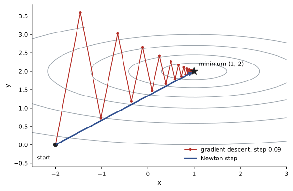
The output shows the trade-off clearly. The largest stable step for gradient descent is set by the steepest direction (here \(\alpha < 2/20 = 0.1\)), and progress along the shallow direction is then slow. Rescaling the variables so that the bowl is round, called preconditioning, is one of the most effective tricks in numerical optimization, and it is the same idea as choosing good units and dimensionless variables.
Common mistakes
MistakeChecking only interior critical points for absolute extremes.
InsteadAlso examine the boundary and compare all candidates.
MistakeConcluding a minimum from positive diagonal entries of the Hessian alone.
InsteadCheck that all eigenvalues are positive (or use D > 0 with f_xx > 0 in two variables).
MistakeTreating the Lagrange multiplier as meaningless.
Insteadλ is the sensitivity of the optimum to the constraint level.
MistakeOptimizing before agreeing on the objective.
InsteadStiffness, strength and cost give different optima; decide what matters first.
MistakeUsing too large a step in gradient descent.
InsteadThe step must be below 2 divided by the largest Hessian eigenvalue, or the iteration diverges.
Summary and key terms
- The second-order Taylor expansion involves the symmetric Hessian matrix H.
- At a critical point, the signs of the eigenvalues of H decide minimum, maximum or saddle.
- Absolute extremes on a closed region occur at interior critical points or on the boundary.
- Least squares minimizes the sum of squared errors and leads to the normal equations.
- The Lagrange multiplier equals df*/dc, the sensitivity of the optimum to the constraint.
- Two constraints need two multipliers; inequality constraints are either active or inactive (KKT).
- Gradient descent is simple but slow in narrow valleys; Newton's method uses the Hessian and converges fast.
- Hessian matrix
- The symmetric matrix of second partial derivatives.
- Positive definite
- A symmetric matrix whose eigenvalues are all positive.
- Absolute extreme
- The largest or smallest value of a function over a whole region.
- Normal equations
- The linear equations whose solution gives the least-squares fit.
- Shadow price
- The value of a Lagrange multiplier as the marginal worth of relaxing a constraint.
- Active constraint
- An inequality constraint that holds with equality at the optimum.
- KKT conditions
- The optimality conditions for problems with inequality constraints.
- Gradient descent
- An iterative method that steps opposite the gradient.
- Newton's method
- An iterative method that uses the gradient and Hessian to jump to the minimum of a local quadratic model.
- Preconditioning
- Rescaling a problem so that numerical methods converge faster.
Practice problems
Work each problem on paper first, then reveal the answer to check.
Find the Hessian of \(f = x^2y + y^3\) at (1, 1).
Show answer
[[2, 2], [2, 6]].
Classify the critical point of \(f = x^2 + 4xy + y^2\) at the origin.
Show answer
H = [[2, 4], [4, 2]], eigenvalues 6 and −2: saddle.
Is \(H = \begin{pmatrix} 2 & 1 \\ 1 & 2 \end{pmatrix}\) positive definite?
Show answer
Yes; eigenvalues 3 and 1.
Find the absolute maximum of \(f = x + y\) on the disc \(x^2 + y^2 \le 4\).
Show answer
2√2 at (√2, √2).
Fit y = mx + c to (0, 0), (1, 1), (2, 4).
Show answer
5m + 3c = 9, 3m + 3c = 5: m = 2, c = −1/3.
For the can example, what are r and h for V = 500 cm³?
Show answer
r = (500/2π)^(1/3) = 4.30 cm, h = 8.60 cm.
Maximize \(f = xyz\) subject to \(x + y + z = 12\), x, y, z > 0.
Show answer
x = y = z = 4, f = 64.
In that problem, what is λ and what does it mean?
Show answer
λ = yz = 16: f* rises by about 16 per unit increase in the sum.
What is the largest stable gradient descent step for \(f = x^2 + 25y^2\)?
Show answer
Hessian eigenvalues 2 and 50: α < 2/50 = 0.04.
How many Newton steps minimize a quadratic function exactly?
Show answer
One.
Lesson quiz · 5 questions
Score 60% or more to complete this lesson.
Create a free account to save your progress, take quizzes and earn a certificate.