An introduction to the finite element method

Finite differences work beautifully on rectangular grids, but engineering parts are not rectangles: a bracket with holes and fillets, a turbine blade, a dam on an irregular valley, a bone, a car body. The finite element method (FEM) handles such shapes by dividing the region into simple pieces (elements), approximating the solution by a simple function on each, and assembling the pieces into one large sparse system. It is the basis of the structural, thermal and electromagnetic analysis software used throughout engineering. This lesson develops the method in one dimension, where every step can be done by hand: the weak form of the governing equation, piecewise linear shape functions, element stiffness matrices and load vectors, assembly, boundary conditions and convergence. It then explains how the same ideas extend to two and three dimensions, and what an engineer must understand to use commercial FEM software responsibly.

The model problem: an axially loaded bar

A bar along \(0 \le x \le L\) with axial stiffness EA(x) carries a distributed axial load f(x) (such as its own weight). Equilibrium of a short slice gives the differential equation for the axial displacement u(x):

with, for example, a fixed end \(u(0) = 0\) and an end load \(EA\,u'(L) = P\). The same equation, with different symbols, governs steady heat conduction along a rod (temperature, conductivity, heat source), seepage through a soil column and electrostatics in one dimension, so everything below applies to those too.

The weak form

Instead of requiring the equation to hold at every point, multiply it by an arbitrary test function v(x) that is zero where u is prescribed, and integrate over the bar. Integrating the left side by parts (MATH-101) moves one derivative onto v:

This weak form must hold for every admissible v. It needs only first derivatives of u, so it admits approximations that are merely continuous, with kinks at element boundaries. The end load appears automatically in the boundary term: conditions on the derivative (forces, heat fluxes) are natural boundary conditions, satisfied by the weak form itself, while conditions on the value (fixed displacements, set temperatures) are essential boundary conditions, imposed directly on the unknowns. For elastic problems, the weak form is exactly the principle of virtual work, so it has a direct physical meaning: internal virtual work equals external virtual work for every virtual displacement.

Elements and shape functions

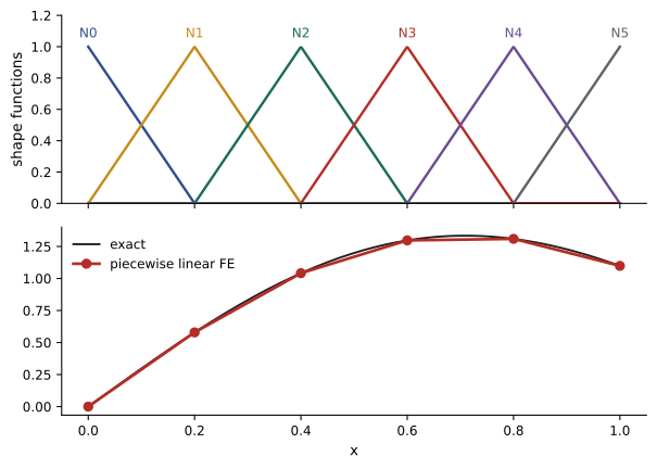
Divide the bar into elements between nodes \(x_0, x_1, \ldots, x_n\), and approximate u by a continuous function that is linear on each element. Such a function is determined by its nodal values \(u_j\):

where the shape function \(N_j\) is the hat function that equals 1 at node j, 0 at all other nodes, and is linear in between. The Galerkin method uses the same hat functions as test functions. Substituting into the weak form with \(v = N_i\), for each free node i, gives a linear system \(K\mathbf{u} = \mathbf{F}\) with

Because each hat function is non-zero only on the two elements touching its node, \(K_{ij}\) is zero unless nodes i and j share an element. The stiffness matrix is therefore sparse (tridiagonal in one dimension), symmetric and, once the essential conditions are applied, positive definite (MATH-125).

Element matrices and assembly

In practice K is not computed entry by entry. Each element of length h contributes only to its own two nodes. On an element with constant EA, the shape function derivatives are \(\mp 1/h\), and the element stiffness matrix and load vector (for a uniform load f) are

This is simply a spring of stiffness EA/h between two nodes, with the element's load shared equally. Assembly adds each element matrix into the rows and columns of the global matrix that correspond to its nodes. Essential conditions are then applied, typically by deleting the rows and columns of fixed degrees of freedom, and the system is solved. Afterwards, element strains and stresses are recovered from the nodal displacements: in each element, \(\varepsilon = (u_{right} - u_{left})/h\).

Convergence

With linear elements of size h, the error in displacement falls as \(h^2\) and the error in stress (a derivative) as h, provided the exact solution is smooth. Refining the mesh (h-refinement) or using higher-order elements, quadratic or cubic (p-refinement), improves accuracy. The code below models a tapered bar, where EA varies along the length and the nodal values are no longer exact, and shows the expected convergence.

import numpy as np

# Tapered steel bar: area falls linearly from A0 at the support to A0/2 at the free end, end load P
E, A0, L, P = 200e9, 4e-4, 2.0, 50e3
exact_tip = P * 2 * L * np.log(2) / (E * A0)

def fe_bar(n):
    h = L / n
    K = np.zeros((n + 1, n + 1))
    F = np.zeros(n + 1)
    for e in range(n):
        xm = (e + 0.5) * h
        EA = E * A0 * (1 - xm / (2 * L))          # stiffness at the element midpoint
        k = EA / h * np.array([[1.0, -1.0], [-1.0, 1.0]])
        K[e:e + 2, e:e + 2] += k                   # assembly
    F[-1] = P                                      # end load at the last node
    u = np.zeros(n + 1)
    u[1:] = np.linalg.solve(K[1:, 1:], F[1:])      # node 0 is fixed: remove its row and column
    return u[-1]

prev = None
for n in [1, 2, 4, 8, 16]:
    tip = fe_bar(n)
    err = abs(tip - exact_tip)
    ratio = f"{prev / err:5.2f}" if prev else "   --"
    print(f"{n:2d} elements: tip displacement {tip * 1000:.5f} mm, error {err * 1000:.2e} mm, ratio {ratio}")
    prev = err
print(f"Exact: {exact_tip * 1000:.5f} mm")

 1 elements: tip displacement 1.66667 mm, error 6.62e-02 mm, ratio    --
 2 elements: tip displacement 1.71429 mm, error 1.86e-02 mm, ratio  3.56
 4 elements: tip displacement 1.72805 mm, error 4.82e-03 mm, ratio  3.86
 8 elements: tip displacement 1.73165 mm, error 1.22e-03 mm, ratio  3.96
16 elements: tip displacement 1.73256 mm, error 3.05e-04 mm, ratio  3.99
Exact: 1.73287 mm

The error falls by four with each doubling of the element count, and 16 elements give the tip displacement to within 0.02%. One element is too stiff, as finite element models with too few elements usually are: the displacement-based method always underestimates the true flexibility, so coarse models predict deflections that are too small.

Two and three dimensions

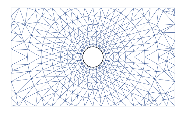
In two dimensions the region is divided into triangles or quadrilaterals, and in three into tetrahedra or bricks. Shape functions are linear (or higher-order) polynomials on each element, equal to 1 at one node and 0 at the others, exactly as in one dimension. The weak form of the governing equation, for instance the equilibrium of an elastic solid or steady heat conduction, gives element matrices by integrating products of shape-function derivatives over each element, usually by Gauss quadrature (Lesson 7) on a reference element mapped to the real one with a Jacobian (MATH-209). Assembly, boundary conditions and the sparse solve are the same, only larger: a model with a million nodes and three displacements per node has three million unknowns, solved with the sparse direct or iterative methods of Lesson 3. Vibration analysis adds a mass matrix and solves \(K\boldsymbol{\phi} = \omega^2M\boldsymbol{\phi}\) by the Lanczos methods of Lesson 4; transient heat flow adds a capacity matrix and steps in time with the schemes of Lesson 10.

Using finite element software responsibly

Commercial and open-source programs (ANSYS, Abaqus, COMSOL, CalculiX, Code_Aster, FEniCS and others) automate meshing, assembly and solution, and produce persuasive color plots. The engineer remains responsible for the result. Good practice includes:

• Check equilibrium: reactions should balance the applied loads.
• Refine the mesh where results vary quickly (near holes, fillets and loads) and confirm that the quantities of interest converge.
• Beware singularities: at a sharp re-entrant corner or a point load, the theoretical stress is infinite, and refining the mesh makes the computed peak grow without limit. Read stresses away from such points, or model the real fillet radius.
• Use appropriate element types: thin plates and shells, beams and nearly incompressible materials such as rubber need special formulations, or results can be grossly too stiff (locking).
• Validate against hand calculations, simple beam or pressure-vessel formulas, or test data.