Computing eigenvalues

Eigenvalue problems are everywhere in engineering. The natural frequencies and mode shapes of a building, bridge or aircraft wing are eigenvalues and eigenvectors of its stiffness and mass matrices; the buckling loads of a frame are eigenvalues; the stability of a control system or a power grid depends on the eigenvalues of its system matrix; principal stresses and principal axes are eigenvalues of a symmetric tensor; and the long-run behavior of a Markov chain, including the ranking of web pages, is an eigenvector. MATH-125 found eigenvalues by solving the characteristic polynomial, which works for 2 × 2 and 3 × 3 matrices but is hopeless for the thousands or millions of unknowns in a finite element model. This lesson develops the methods computers actually use: power iteration, inverse iteration with shifts, the Rayleigh quotient, the QR algorithm behind every library eigenvalue routine, and the Krylov methods that find a few eigenvalues of huge sparse matrices. It also explains when computed eigenvalues can be trusted.

Why not the characteristic polynomial?

For an n × n matrix, \(\det(A - \lambda I) = 0\) is a polynomial of degree n. Expanding the determinant costs far more than solving the eigenvalue problem directly, and there is a deeper problem: the roots of a polynomial can be extremely sensitive to its coefficients. Wilkinson's famous example has roots 1, 2, …, 20; changing one coefficient by about one part in 10¹⁰ moves several roots by large amounts and makes some of them complex. Round-off in forming the coefficients (Lesson 1) is enough to ruin the answer. So numerical methods never form the characteristic polynomial; instead they work with the matrix itself, using operations that keep errors small. In fact, the reverse is true: library routines find the roots of a polynomial by computing the eigenvalues of a matrix built from its coefficients.

Power iteration

The simplest method repeatedly multiplies a starting vector by A and normalizes:

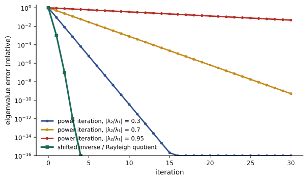
To see why this works, write the starting vector as a combination of eigenvectors, \(\mathbf{x}_0 = c_1\mathbf{v}_1 + c_2\mathbf{v}_2 + \cdots\). After k multiplications the components have been scaled by \(\lambda_1^k, \lambda_2^k, \ldots\). If \(|\lambda_1|\) is strictly the largest, its component dominates, and \(\mathbf{x}_k\) turns toward \(\mathbf{v}_1\). The error shrinks by a factor of about \(|\lambda_2/\lambda_1|\) at each step, so convergence is fast when the dominant eigenvalue is well separated and slow when it is not.

The best estimate of the eigenvalue from an approximate eigenvector is the Rayleigh quotient:

For a symmetric matrix, its error is proportional to the square of the error in the vector, so it converges twice as fast as the vector does.

Power iteration needs only matrix-vector products, so it works for enormous sparse matrices. Google's original PageRank computed the dominant eigenvector of a matrix describing links among billions of web pages in exactly this way. Its weakness is that it finds only the largest eigenvalue, while engineers usually want the smallest: the fundamental frequency or the lowest buckling load.

Inverse iteration and shifts

The eigenvalues of \(A^{-1}\) are \(1/\lambda_i\), with the same eigenvectors, so power iteration applied to \(A^{-1}\) finds the eigenvalue of A closest to zero. More generally, the eigenvalues of \((A - \sigma I)^{-1}\) are \(1/(\lambda_i - \sigma)\), so power iteration with this matrix finds the eigenvalue closest to the shift σ, and converges at the rate \(|\lambda_{near} - \sigma|/|\lambda_{next} - \sigma|\), which can be made very small with a good shift. The inverse is never formed: each step solves \((A - \sigma I)\mathbf{y} = \mathbf{x}_k\), using an LU factorization (Lesson 3) computed once and reused, so each step costs only a forward and back substitution.

Updating the shift at every step to the latest Rayleigh quotient gives Rayleigh quotient iteration, which for symmetric matrices converges cubically: the number of correct digits roughly triples each step, at the cost of refactoring the matrix each time.

import numpy as np
from scipy.linalg import eigh, lu_factor, lu_solve

# Ten-storey shear building: floor mass 50 t, storey stiffness 40 MN/m
n, m, k = 10, 50e3, 40e6
K = np.zeros((n, n))
for i in range(n):
    K[i, i] = 2 * k if i < n - 1 else k
    if i > 0:
        K[i, i - 1] = K[i - 1, i] = -k
A = K / m                                  # equal masses, so K phi = w^2 M phi becomes A phi = w^2 phi

def power(A, iters):
    x = np.ones(len(A))
    for _ in range(iters):
        x = A @ x
        x = x / np.linalg.norm(x)
    return x @ A @ x, x

def inverse(A, shift, iters):
    lu = lu_factor(A - shift * np.eye(len(A)))   # factor once, reuse every step
    x = np.ones(len(A))
    for _ in range(iters):
        x = lu_solve(lu, x)
        x = x / np.linalg.norm(x)
    return x @ A @ x, x

hz = lambda lam: np.sqrt(lam) / (2 * np.pi)
lam_all = eigh(A, eigvals_only=True)
print("Exact (eigh):        f1 = %.4f Hz, f2 = %.4f Hz, f10 = %.3f Hz" % (hz(lam_all[0]), hz(lam_all[1]), hz(lam_all[-1])))
for it in [5, 20, 100]:
    lam, _ = power(A, it)
    print(f"Power, {it:3d} steps:    highest f = {hz(lam):.3f} Hz")
for it in [3, 10]:
    lam, x = inverse(A, 0.0, it)
    print(f"Inverse, {it:2d} steps:   lowest f = {hz(lam):.4f} Hz")
lam, x = inverse(A, (2 * np.pi * 1.9)**2, 5)
print(f"Shifted inverse near 1.9 Hz, 5 steps: f = {hz(lam):.4f} Hz")

Exact (eigh):        f1 = 0.6728 Hz, f2 = 2.0034 Hz, f10 = 8.903 Hz
Power,   5 steps:    highest f = 8.367 Hz
Power,  20 steps:    highest f = 8.836 Hz
Power, 100 steps:    highest f = 8.903 Hz
Inverse,  3 steps:   lowest f = 0.6728 Hz
Inverse, 10 steps:   lowest f = 0.6728 Hz
Shifted inverse near 1.9 Hz, 5 steps: f = 2.0034 Hz

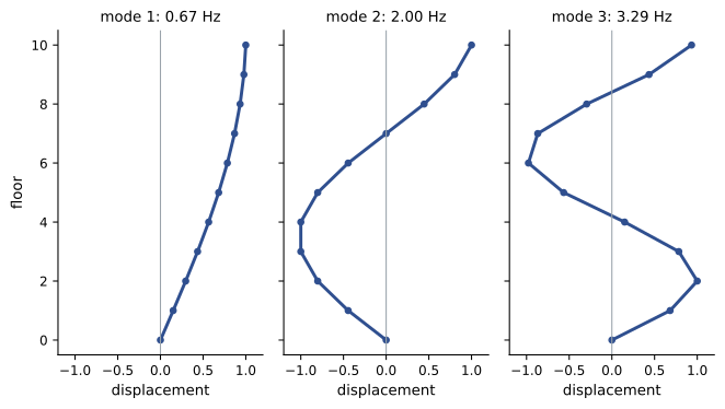
Power iteration needs about 100 steps for the highest frequency, because the top two eigenvalues are close; inverse iteration finds the fundamental frequency, 0.673 Hz, in three steps, and a shift near 1.9 Hz picks out the second mode just as quickly. Structural engineers care most about the lowest few modes, which dominate earthquake and wind response, so shifted inverse methods are the workhorses of structural dynamics.

The QR algorithm

To find all the eigenvalues of a dense matrix, libraries such as LAPACK (used by NumPy, MATLAB and others) use the QR algorithm. Factor \(A_0 = A\) as \(A_0 = Q_0R_0\), with Q orthogonal and R upper triangular (MATH-125), then multiply in the reverse order: \(A_1 = R_0Q_0\). Since \(A_1 = Q_0^TA_0Q_0\), it has the same eigenvalues. Repeating, the matrices \(A_k\) converge (under mild conditions) to an upper triangular matrix, with the eigenvalues appearing on the diagonal. The practical algorithm adds three refinements that make it fast and reliable:

• First reduce A to Hessenberg form (zeros below the first subdiagonal), or tridiagonal form if A is symmetric, using orthogonal transformations. Each QR step then costs \(O(n^2)\) instead of \(O(n^3)\).
• Use shifts, \(A_k - \sigma_kI = Q_kR_k\), \(A_{k+1} = R_kQ_k + \sigma_kI\), chosen from the bottom corner of the matrix, so that each eigenvalue converges in two or three steps.
• Deflate: once a subdiagonal entry is negligible, split the problem and continue on the smaller pieces.

The whole process costs about \(10n^3\) operations for all eigenvalues and eigenvectors of a general matrix, fewer for a symmetric one. A 1000 × 1000 problem takes well under a second on a laptop; a 100 000 × 100 000 dense problem would take days and 80 GB of memory, which is why large problems use the methods below.

Symmetric and generalized problems

Most engineering eigenvalue problems are symmetric, because stiffness and mass matrices, covariance matrices and stress tensors are symmetric. Symmetric problems are easier and better behaved: the eigenvalues are real, the eigenvectors can be chosen orthogonal, and the eigenvalues are well conditioned, meaning that a perturbation of size ε in the matrix moves each eigenvalue by at most ε. Use the routines for symmetric matrices (numpy.linalg.eigh or scipy.linalg.eigh) rather than the general ones; they are faster and guarantee real results.

Vibration problems usually come in generalized form, \(K\boldsymbol{\phi} = \omega^2M\boldsymbol{\phi}\). It is tempting to form \(M^{-1}K\), but that matrix is not symmetric. Instead, solvers either pass both matrices to a generalized routine (scipy.linalg.eigh(K, M)) or use a Cholesky factorization \(M = LL^T\) to convert the problem to a standard symmetric one.

Large sparse problems

A finite element model of a car body or an aircraft may have millions of unknowns, but its matrices are sparse, and only the lowest few dozen modes are needed. Krylov subspace methods (Lanczos for symmetric matrices, Arnoldi for general ones) build a small basis from the vectors \(\mathbf{x}, A\mathbf{x}, A^2\mathbf{x}, \ldots\), whose span captures the extreme eigenvalues remarkably well, and solve a small eigenvalue problem within it. Combined with the shift-and-invert idea, so that the eigenvalues near a chosen σ become the extreme ones, they find the lowest modes of enormous models efficiently. In Python this is scipy.sparse.linalg.eigsh, which wraps the ARPACK library used by many commercial programs.

Checking computed eigenvalues

A computed pair \((\lambda, \mathbf{x})\) can always be checked through its residual, \(\|A\mathbf{x} - \lambda\mathbf{x}\|/\|\mathbf{x}\|\). For a symmetric matrix, a small residual guarantees that some true eigenvalue lies within that distance of λ. Further checks come from physics: the sum of the eigenvalues equals the trace of A; mode shapes should be orthogonal with respect to the mass matrix; the lowest frequency should be consistent with a simple hand estimate; and refining a finite element mesh should change the lowest frequencies only slightly.