Case studies and course project

This course has assembled a toolkit of numerical methods: floating-point arithmetic and error analysis, root finding, linear systems, eigenvalues, interpolation and fitting, optimization, quadrature, ODE solvers for initial and boundary value problems, finite differences for PDEs and the finite element method. In practice these tools are combined, and the skill lies in choosing them, chaining them together and checking the result. This lesson works through three case studies of that kind: diagnosing a machine fault from a vibration signal with the fast Fourier transform, quantifying how uncertain inputs affect a design calculation with Monte Carlo simulation, and predicting the quench time of a steel plate by two independent methods that check each other. It then sets out the course project and the habits of verification that make numerical results trustworthy.

Case study 1: vibration monitoring with the FFT

Rotating machines announce developing faults through their vibration: an unbalanced rotor vibrates at the running speed, a misaligned coupling at twice it, and damaged bearings at characteristic frequencies set by their geometry. Condition monitoring systems record accelerometer signals and look for these frequencies in the spectrum.

The discrete Fourier transform (DFT) of N samples \(x_0, \ldots, x_{N-1}\) taken at sampling rate \(f_s\) is

It expresses the record as a sum of sinusoids, the discrete counterpart of the Fourier series of MATH-201. Computed directly it costs \(O(N^2)\) operations; the fast Fourier transform (FFT) reorganizes the sum recursively and costs \(O(N\log N)\), so a million-point spectrum takes milliseconds instead of hours. The FFT is one of the most important algorithms ever devised, used in signal processing, imaging, communications and the fast solution of PDEs.

Three practical rules govern its use. The highest frequency that can be represented is the Nyquist frequency \(f_s/2\); higher frequencies in the signal fold back as false low frequencies (aliasing), so signals are filtered before sampling and sampled at more than twice the highest frequency of interest. The frequency resolution is \(1/T\), the reciprocal of the record length, so separating close frequencies needs long records. And a finite record cuts sinusoids off abruptly, which smears their energy into neighboring frequencies (leakage); multiplying the record by a smooth window, such as the Hann window, reduces this.

import numpy as np
from scipy.signal import find_peaks

# Vibration signal from a pump bearing: running speed 29.5 Hz, a fault tone at 107 Hz, plus noise
fs, T = 1000.0, 4.0                       # sampling rate (Hz) and record length (s)
t = np.arange(0, T, 1 / fs)
rng = np.random.default_rng(3)
signal = 1.0 * np.sin(2 * np.pi * 29.5 * t) + 0.15 * np.sin(2 * np.pi * 107.0 * t) + 0.5 * rng.normal(size=t.size)

window = np.hanning(t.size)               # reduces leakage from the finite record
spectrum = np.abs(np.fft.rfft(signal * window)) * 2 / window.sum()
freqs = np.fft.rfftfreq(t.size, 1 / fs)
print(f"{t.size} samples, frequency resolution {freqs[1]:.2f} Hz, Nyquist frequency {fs / 2:.0f} Hz")
peaks, _ = find_peaks(spectrum, height=0.08)
for i in peaks:
    print(f"Peak at {freqs[i]:6.2f} Hz, amplitude {spectrum[i]:.3f}")
print(f"Median noise level in the spectrum: {np.median(spectrum):.4f}")

4000 samples, frequency resolution 0.25 Hz, Nyquist frequency 500 Hz
Peak at  29.50 Hz, amplitude 1.004
Peak at 107.00 Hz, amplitude 0.164
Median noise level in the spectrum: 0.0163

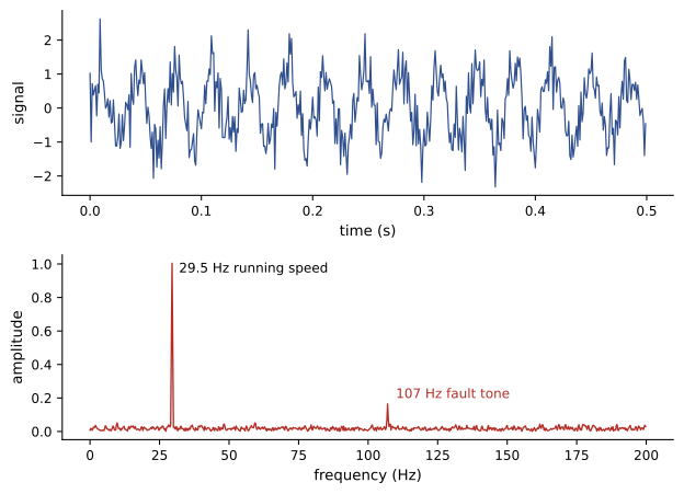
In the time record, the fault tone is completely buried: its amplitude is less than a third of the noise standard deviation. In the spectrum it stands out at about ten times the noise floor, because the FFT concentrates a steady tone into a single frequency bin while spreading random noise across all 2000 bins. Tracking such peaks over weeks lets maintenance be planned before a bearing fails.

Case study 2: uncertainty in a design calculation

Every input to an engineering calculation is uncertain: loads vary, material properties scatter, dimensions have tolerances. How uncertain is the answer? Two numerical approaches complement each other. The first-order (linearized) method uses partial derivatives: for a product of powers such as \(d \propto wL^4/(EI)\), the relative standard deviations combine as

assuming independent inputs (STAT-235 develops this). Monte Carlo simulation instead samples all the inputs at random many times, evaluates the model for each sample and studies the distribution of results. It handles nonlinear models, correlated inputs and probabilities of exceeding a limit, at the cost of many model evaluations, with errors falling as \(1/\sqrt{N}\) (MATH-209).

import numpy as np

# Midspan deflection of a simply supported beam: d = 5 w L^4 / (384 E I), with uncertain inputs
rng = np.random.default_rng(7)
n = 200_000
w = rng.normal(12e3, 1.2e3, n)          # load, N/m (10% coefficient of variation)
E = rng.normal(200e9, 10e9, n)          # modulus, Pa (5%)
I = rng.normal(1.6e-4, 0.08e-4, n)       # second moment, m^4 (5%)
L = rng.normal(8.0, 0.02, n)            # span, m
d = 5 * w * L**4 / (384 * E * I) * 1000 # mm

d0 = 5 * 12e3 * 8.0**4 / (384 * 200e9 * 1.6e-4) * 1000
cov = np.sqrt(0.10**2 + 0.05**2 + 0.05**2 + (4 * 0.02 / 8.0)**2)   # first-order estimate
print(f"Nominal deflection {d0:.2f} mm")
print(f"Monte Carlo: mean {d.mean():.2f} mm, standard deviation {d.std():.2f} mm")
print(f"First-order estimate of standard deviation: {d0 * cov:.2f} mm")
print(f"Probability that deflection exceeds L/360 = {8000 / 360:.1f} mm: {np.mean(d > 8000 / 360):.4f}")

Nominal deflection 20.00 mm
Monte Carlo: mean 20.10 mm, standard deviation 2.47 mm
First-order estimate of standard deviation: 2.46 mm
Probability that deflection exceeds L/360 = 22.2 mm: 0.1915

The first-order standard deviation matches the Monte Carlo result closely here, because the model is smooth and the uncertainties modest. The Monte Carlo run adds what the linear method cannot easily give: the probability, about 19%, that the deflection exceeds the serviceability limit of span/360 even though the nominal value of 20 mm satisfies it. The load uncertainty dominates, so better load information would narrow the result more than a better modulus. Design codes handle such uncertainty with load and resistance factors calibrated by exactly this kind of reliability analysis.

Case study 3: quenching a steel plate

A steel plate 50 mm thick, at 850 °C, is quenched in oil at 60 °C. Metallurgists need to know when the center falls below 300 °C. With conductivity k = 45 W/(m·K), diffusivity α = 1.2 × 10⁻⁵ m²/s and a heat transfer coefficient h = 500 W/(m²·K), heat conducts to the surfaces and is removed by convection there. The Biot number \(Bi = hb/k = 0.278\), with b the half-thickness, measures the resistance to heat transfer at the surface relative to conduction inside.

Two independent methods are used. The first is the classical one-term series solution for a slab with convective surfaces, whose decay rate depends on the first root of \(\lambda\tan\lambda = Bi\), a transcendental equation solved by root finding (Lesson 2). The second is a Crank-Nicolson finite difference model (Lesson 10) of the half-thickness, with a symmetry condition at the center and a convective (Robin) condition at the surface, \(-k\,\partial T/\partial x = h(T - T_{oil})\), both imposed with ghost points (Lesson 9). The time at which the center crosses 300 °C is found by linear interpolation between steps.

import numpy as np
from scipy.linalg import solve_banded
from scipy.optimize import brentq

# Oil quench of a steel plate 50 mm thick: half-thickness b = 25 mm, mid-plane insulated by symmetry
k, alpha, h_c, b = 45.0, 1.2e-5, 500.0, 0.025
T0, Toil, target = 850.0, 60.0, 300.0
Bi = h_c * b / k

# One-term series: lambda tan(lambda) = Bi, found by root finding
lam = brentq(lambda z: z * np.tan(z) - Bi, 1e-6, np.pi / 2 - 1e-6)
C1 = 4 * np.sin(lam) / (2 * lam + np.sin(2 * lam))
theta = (target - Toil) / (T0 - Toil)
t_series = -np.log(theta / C1) / lam**2 * b**2 / alpha
print(f"Biot number {Bi:.3f}, first eigenvalue {lam:.4f}, one-term time {t_series:.1f} s")

# Crank-Nicolson finite differences with a convective (Robin) surface and ghost points at both ends
N, dt = 50, 0.25
dx = b / N
r = alpha * dt / dx**2
beta = 2 * dx * h_c / k
A = np.zeros((N + 1, N + 1))
for i in range(N + 1):
    A[i, i] = -2.0
    if i > 0:
        A[i, i - 1] = 1.0
    if i < N:
        A[i, i + 1] = 1.0
A[0, 1] = 2.0                        # symmetry at the mid-plane
A[N, N - 1] = 2.0; A[N, N] = -2.0 - beta
src = np.zeros(N + 1); src[N] = beta * Toil
M_left = np.eye(N + 1) - 0.5 * r * A
M_right = np.eye(N + 1) + 0.5 * r * A
ab = np.zeros((3, N + 1))
ab[0, 1:] = np.diag(M_left, 1); ab[1] = np.diag(M_left); ab[2, :-1] = np.diag(M_left, -1)

T = np.full(N + 1, T0); t = 0.0
while T[0] > target:
    T_old, t_old = T.copy(), t
    T = solve_banded((1, 1), ab, M_right @ T + r * src)
    t += dt
t_fd = t_old + dt * (T_old[0] - target) / (T_old[0] - T[0])
print(f"Finite differences: mid-plane reaches {target:.0f} C after {t_fd:.1f} s; surface then at {T[-1]:.0f} C")

Biot number 0.278, first eigenvalue 0.5038, one-term time 252.9 s
Finite differences: mid-plane reaches 300 C after 252.9 s; surface then at 270 C

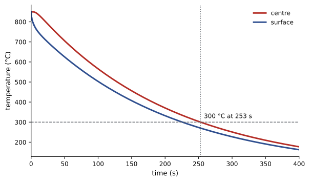
The two methods agree to within a tenth of a second, at about 253 s, which gives strong confidence in both. The finite difference model can now be trusted for what the series cannot do: a heat transfer coefficient that changes as the oil boils at the surface, temperature-dependent properties, or a plate of varying thickness. This is the pattern of good numerical practice: build confidence on a case with an independent check, then extend the model.

Verification habits

The case studies share habits that apply to all numerical work:

• Know the expected answer roughly before computing it: an order-of-magnitude estimate, a limiting case, a one-term series.
• Check convergence: refine the grid, tighten the tolerance or increase the samples, and confirm that the answer settles at the expected rate.
• Use an independent method on at least one case: a different algorithm, an analytical solution or a measurement.
• Check conservation and balance: energy, mass, forces, probability.
• Understand the conditioning of the problem (Lesson 1): no algorithm can deliver more accuracy than the data and the problem allow.
• Record versions, inputs and settings so that results can be reproduced.

The course project

Choose one of the following problems, or propose your own of similar scope with your instructor's approval. Write your own code (Python is recommended) and prepare a report with the formulation, the methods and why they were chosen, verification, results and interpretation.

• Project A: Structural dynamics. Model a multi-story frame or a beam with springs and masses, compute its natural frequencies and modes with your own inverse iteration and with a library solver, then simulate its response to a recorded or synthetic ground motion with an adaptive ODE solver. Check the energy balance and the effect of damping.
• Project B: Heat transfer. Solve a transient conduction problem with a convective boundary in one or two dimensions using an implicit scheme, verify it against an analytical solution, and use it with root finding or optimization to answer a design question (insulation thickness, quench time, heating schedule).
• Project C: Data and models. Obtain an engineering data set (a calibration curve, a pump test, a stress-strain curve, a cooling curve). Fit linear and nonlinear models by least squares, compare them with residual analysis and cross-validation, and quantify parameter uncertainty by bootstrap or Monte Carlo.
• Project D: Finite elements. Write a one-dimensional finite element code for a bar, rod or beam with varying properties, verify its convergence rate against an exact solution, and compare one result with a commercial or open-source two-dimensional program.

Every report should state the governing equations and assumptions, justify each numerical choice (method, grid, tolerance), present a convergence study and an independent check, discuss the main sources of error and uncertainty, and end with clear engineering conclusions.

Looking ahead

Numerical methods are the engine behind computational engineering: finite element analysis in structural and mechanical design, computational fluid dynamics in aerospace, energy and environmental work, circuit simulation in electrical engineering, process simulation in chemical engineering, and data analysis and machine learning everywhere. Later courses will use these methods, often through large software packages, and the understanding built here, of accuracy, stability, conditioning, cost and verification, is what lets an engineer use those packages with judgment rather than blind trust.