Kinematics of particles: rectilinear motion

Statics, the subject of ENGG-130, deals with bodies that are at rest or moving at constant velocity, where the forces balance. Dynamics deals with everything else: the shuttle that accelerates down an aisle of a warehouse, the parcel that flies off the end of a chute, the crank that drives a pump, the robot arm that swings a payload into a bin, the car suspension that bounces over a pothole. Almost every machine a mechanical engineer designs has parts that accelerate, and the forces that cause those accelerations are often far larger than the static loads. Getting the dynamics right is the difference between a machine that runs smoothly for years and one that shakes itself apart, throws its load or fails the first time someone presses the emergency stop.

Dynamics has two halves. Kinematics is the geometry of motion: how position, velocity and acceleration are related, without asking what causes the motion. Kinetics connects motion to its causes, the forces and moments, through Newton's laws and the work-energy and impulse-momentum principles derived from them. This course follows the usual order. Lessons 1 to 3 cover the kinematics of particles, Lessons 4 to 7 the kinetics of particles, Lessons 8 and 9 the kinematics of rigid bodies, Lessons 10 and 11 their kinetics, and Lesson 12 introduces vibration, where everything comes together.

Throughout the course we follow the engineers of Kestrel Automation, an invented systems integrator in Columbus, Ohio, that designs conveyors, sorters, tote shuttles and robotic cells for distribution centers. Anika Sharma, PE, leads the mechanical team; Tomás Reyes is an engineer intern (EI) who has just joined it. Their current project is a parcel sorting hall for a regional distribution center, and nearly every topic in this course turns up somewhere in it. Most calculations use SI units, which dominate machine design and textbooks, but each lesson also works an example in US customary units (feet, pounds and slugs), because many American drawings, codes and catalogs still use them.

Particles and reference frames

A particle is a body whose size and rotation do not matter for the question being asked. A 30 kg tote on a shuttle can be treated as a particle when we want to know how long it takes to travel 18 m, even though it has a definite size, because every point on it moves the same way. The same tote cannot be treated as a particle if we want to know whether it will tip over when the shuttle brakes, because then its rotation matters. The particle model is a choice the engineer makes, not a property of the object, and part of the skill of dynamics is choosing the simplest model that still answers the question.

Motion is always described relative to a reference frame. For most machine problems the frame is fixed to the ground (the building floor, the machine base) and treated as inertial, meaning that Newton's laws hold in it without correction. The Earth rotates, so a ground frame is not perfectly inertial, but the error is negligible for machines, vehicles and structures. It matters for long-range ballistics, ocean currents and weather, which this course does not cover.

Position, displacement and distance

Rectilinear motion is motion along a straight line. We pick an origin \(O\) on the line and a positive direction, and describe the particle's location by its position coordinate \(s\), which can be positive or negative. If the particle moves from \(s_1\) to \(s_2\), its displacement is \(\Delta s = s_2 - s_1\), a signed quantity. The distance traveled is the total length of path covered, which is always positive and is larger than the size of the displacement whenever the particle reverses direction. A shuttle that goes 10 m down an aisle and comes back 4 m has a displacement of 6 m and has traveled 14 m. The distinction matters in practice: wear on wheels, energy used by drives and cycle counts on bearings all depend on distance traveled, not displacement.

Velocity and acceleration

The average velocity over a time interval \(\Delta t\) is \(\Delta s / \Delta t\). Shrinking the interval to zero gives the instantaneous velocity, the rate of change of position:

The velocity is positive when the particle moves in the positive direction and negative when it moves the other way. Its magnitude is the speed. The acceleration is the rate of change of velocity:

A positive acceleration means the velocity is increasing algebraically. That is not the same as speeding up. A particle moving in the negative direction with a positive acceleration is slowing down. The word deceleration is used loosely for an acceleration that opposes the velocity, and it is safest to avoid it in calculations and keep track of signs instead.

Eliminating \(dt\) between the two definitions gives a third relation that is often the most useful of all, because it connects acceleration to position directly:

These three equations hold for any rectilinear motion. Every problem in this lesson is a matter of choosing the right one, separating variables and integrating, with the initial conditions supplying the constants.

Motion with constant acceleration

When the acceleration is constant, \(a = a_c\), the three relations integrate in closed form. With \(s = s_0\) and \(v = v_0\) at \(t = 0\):

These are the familiar equations from first-year physics, and they are used constantly: a vehicle braking at a steady rate, a body falling freely near the Earth's surface with \(a_c = -g\) (taking up as positive), a drive that ramps a conveyor up to speed at a set rate. Their convenience is also their danger. They apply only when the acceleration is truly constant. A body falling through air, a cam follower, a spring-driven plunger and a vehicle whose engine torque varies with speed all have accelerations that change, and using the constant-acceleration formulas for them gives wrong answers, sometimes badly wrong.

Standard gravity is \(g = 9.81 \text{ m/s}^2\), or \(32.2 \text{ ft/s}^2\). The local value varies by about half a percent between the equator and the poles, which almost never matters in machine design.

The reaction-time term is easy to forget and is often a large part of the answer. In this example it adds about a fifth to the stopping distance. Safety standards for presence-sensing devices require the designer to include the full response time of the sensor, the controller and the brake, and to measure it rather than guess it.

Acceleration that varies

When the acceleration is not constant, it is usually given in one of three forms: as a function of time, of velocity or of position. Each calls for a different relation.

• If \(a = f(t)\), integrate \(dv = f(t)\,dt\) to get \(v(t)\), then \(ds = v(t)\,dt\) to get \(s(t)\).
• If \(a = f(v)\), as with drag forces that grow with speed, separate variables in either \(dt = dv / f(v)\) (to find time) or \(ds = v\,dv / f(v)\) (to find distance).
• If \(a = f(s)\), as with springs and gravitational attraction, use \(v\,dv = f(s)\,ds\) to get velocity as a function of position.

A common error is to integrate \(a = f(s)\) with respect to time, treating \(s\) as a constant. Before integrating, check that the variable in the function matches the variable of integration.

Graphical methods and motion profiles

Because velocity is the slope of the position-time curve and acceleration is the slope of the velocity-time curve, the integrals have simple geometric meanings. The change in velocity over an interval equals the area under the acceleration-time curve, and the change in position equals the area under the velocity-time curve. Engineers who set up motion controllers think in these pictures all the time.

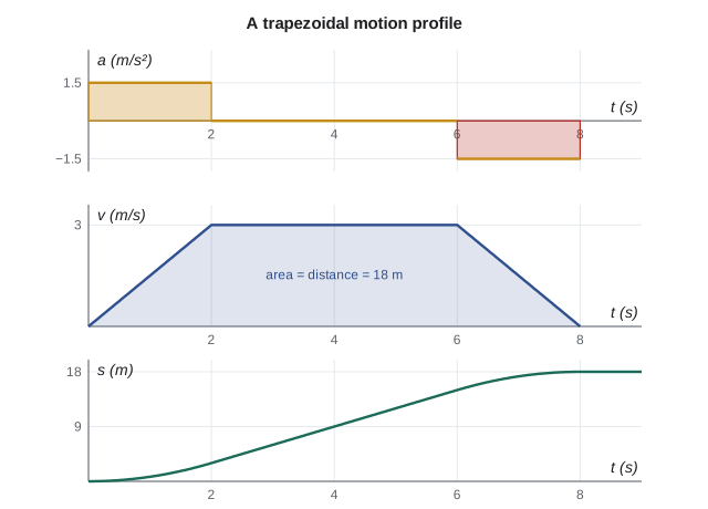
The figure shows the trapezoidal profile used for a typical shuttle move: accelerate at \(1.5 \text{ m/s}^2\) for 2 s to reach 3 m/s, cruise for 4 s, then brake at the same rate for 2 s. The velocity graph is a trapezoid whose area, \(\tfrac12(2)(3) + (4)(3) + \tfrac12(2)(3) = 18 \text{ m}\), is the length of the move. A motion designer working backwards from a required move length, top speed and acceleration limit can size the cruise segment from this area in seconds, without writing a single equation.

The trapezoidal profile has jumps in acceleration at the corners, which means infinite jerk (the rate of change of acceleration) at those instants. Real drives cannot produce that, and attempting it excites vibration in the structure and the load. Most servo controllers therefore offer S-curve profiles, in which the acceleration ramps up and down over a short time. The move takes slightly longer, but the machine runs more quietly and the totes stay put. Lesson 12 returns to why sudden changes in force excite vibration.

Numerical integration

Many real accelerations have no convenient closed-form integral, or are known only as measured data from an accelerometer or a drive log. In those cases the motion is found numerically, by stepping forward in small time increments: from the current velocity and acceleration, estimate the velocity a short time \(\Delta t\) later, then the position, and repeat. The simplest scheme, Euler's method, uses the acceleration at the start of each step; better schemes average values across the step. Whatever the method, the answer should be checked by halving the step and confirming that it barely changes.

The program below models a shuttle coasting to a stop under rolling resistance plus a drag term that grows with the square of speed, \(a = -(c_0 + k v^2)\), with \(c_0 = 0.6 \text{ m/s}^2\), \(k = 0.05 \text{ m}^{-1}\) and an initial speed of 4 m/s. It integrates with three step sizes and compares the results with the exact answer, which comes from separating variables in \(v\,dv = a\,ds\).

# A tote shuttle brakes under aerodynamic-style drag plus rolling resistance:
#   a = -(c0 + k*v^2)   (m/s^2), starting at v0 = 4 m/s.
# Integrate numerically with small time steps and compare the stopping
# distance with the exact answer from a = v dv/ds.
import math

c0, k, v0 = 0.6, 0.05, 4.0          # m/s^2, 1/m, m/s

def accel(v):
    return -(c0 + k * v * v)

for dt in (0.1, 0.01, 0.001):
    t, s, v = 0.0, 0.0, v0
    while v > 0:
        a = accel(v)
        v_new = v + a * dt
        if v_new < 0:                 # stop exactly at v = 0 in the last step
            frac = v / (v - v_new)
            s += v * frac * dt / 2
            t += frac * dt
            break
        s += (v + v_new) / 2 * dt     # trapezoid rule for position
        v, t = v_new, t + dt
    print(f"dt = {dt:<6} stop time = {t:.3f} s   stop distance = {s:.4f} m")

# Exact: v dv/ds = -(c0 + k v^2)  ->  s = ln(1 + k v0^2 / c0) / (2k)
s_exact = math.log(1 + k * v0**2 / c0) / (2 * k)
t_exact = math.atan(v0 * math.sqrt(k / c0)) / math.sqrt(k * c0)
print(f"exact          stop time = {t_exact:.3f} s   stop distance = {s_exact:.4f} m")

dt = 0.1    stop time = 4.905 s   stop distance = 8.3694 m
dt = 0.01   stop time = 4.944 s   stop distance = 8.4627 m
dt = 0.001  stop time = 4.948 s   stop distance = 8.4719 m
exact          stop time = 4.948 s   stop distance = 8.4730 m

With a step of 0.1 s the stopping distance is about 1 percent low; with 0.001 s it agrees with the exact value to about a millimeter. This convergence check is the habit to build: a numerical answer means nothing until you know how it depends on the step size. The exact answer was available here, which made the check easy, but the same program works unchanged for any acceleration function you can compute, including one read from a table of test data.

The exact solution is worth seeing because it shows the method for velocity-dependent acceleration. Separating variables gives

which evaluates to 8.47 m. If the drag term were ignored, the constant-acceleration formula would give \(v_0^2 / (2 c_0) = 13.3 \text{ m}\), more than half as much again. Choosing the right model of acceleration matters more than the algebra that follows.

Units and significant figures

Keep units with every number in a calculation, at least until you are fluent. In US customary units, lengths are in feet, times in seconds, velocities in feet per second and accelerations in feet per second squared. Speeds given in miles per hour must be converted (1 mi/h = 1.467 ft/s), and dimensions given in inches must be divided by 12 before they go into an equation with feet. Report answers to three significant figures unless the data justify more, and carry at least four through intermediate steps so that rounding does not creep into the result.