
ROB-220 · Lesson 1 of 12 · 31 min
Sensor fundamentals: specifications and datasheets
A robot knows only what its sensors tell it, and it can do only what its actuators allow. Every later course in this program, from control to state estimation to manipulation, assumes that you can read a sensor's specifications, predict what its output will look like, and judge whether it is good enough for a job. This first lesson builds that vocabulary. It defines the terms that appear on every datasheet, shows how they combine into an error budget, and practices the habit of asking what a number really means before trusting it. ROB-200 covered the electronics that turn a sensor's voltage into a digital number; here we focus on the sensor itself and on the physical quantity it measures.
What a sensor does
A sensor is a transducer: it converts one physical quantity, the measurand, into another quantity that is easier to process, almost always an electrical signal. A strain gauge turns stretch into a change in resistance; a photodiode turns light into current; a capacitive accelerometer turns acceleration into a change in capacitance. Most practical sensors are packaged with conditioning electronics and a converter, so the robot's computer receives a stream of numbers, but the physics at the front end still sets the limits on what those numbers can tell you.
Robot sensors are usually divided into two families. Proprioceptive sensors measure the robot's own state: joint angles, wheel speeds, motor currents, battery voltage, body acceleration. Exteroceptive sensors measure the world: distances to obstacles, images, contact forces, satellite signals. A second useful division is between passive sensors, which only receive energy that is already present (a camera in daylight, a microphone), and active sensors, which emit energy and measure what comes back (lidar, sonar, radar, structured-light depth cameras). Active sensors work in the dark and give direct range, but they consume power, can interfere with each other and may be subject to emission rules.
A third distinction matters for software: whether the sensor gives an absolute or an incremental reading. An absolute encoder reports the joint angle immediately after power-up; an incremental encoder only counts changes, so the robot must run a homing routine to find a reference. A gyroscope is incremental in a similar sense, because it measures rate of rotation, and angle must be found by integrating, which accumulates error. These differences shape start-up procedures and fault handling as much as the sensors' accuracy does.
The static characteristics
A sensor's static behavior describes its output when the measurand is held constant. The key terms are:
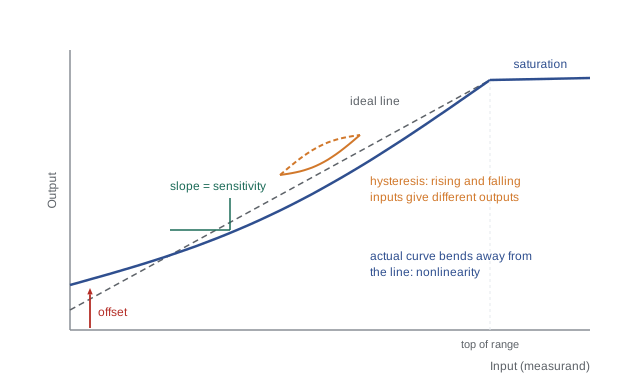
- Range (or span): the interval of input values the sensor can measure, for example 0.05 to 12 m for a small lidar or ±2000 °/s for a gyroscope. Inputs outside the range saturate or give nonsense.
- Sensitivity (or scale factor): the slope of the output against the input, such as 66 mV per ampere for a current sensor or 16.4 counts per °/s for a digital gyroscope. A sensitivity error scales every reading by the same wrong factor.
- Offset (or bias, or zero error): the output when the input is zero. A gyroscope sitting still that reports 0.3 °/s has a bias of 0.3 °/s.
- Resolution: the smallest change in input that produces a detectable change in output. A 4096-count encoder has an angular resolution of 360°/4096 ≈ 0.088°.
- Linearity: how closely the input-output curve follows a straight line, usually quoted as the maximum deviation in percent of full scale (%FS).
- Hysteresis: a difference in output depending on whether the input is rising or falling, common in mechanical and magnetic sensors.
- Repeatability: the spread of readings when the same input is applied many times under the same conditions.
Accuracy, precision and resolution are different things
Three words that are often used loosely deserve precise meanings. Accuracy is how close a reading is to the true value. Precision is how close repeated readings are to each other. Resolution is how finely the output is divided. A sensor can be precise but inaccurate, like a scale that always reads 2 kg heavy; it can be accurate on average but imprecise, with readings scattered around the truth; and it can have fine resolution while being neither accurate nor precise, because extra digits on a display do not make a measurement better. In statistical terms, the systematic part of the error (bias) limits accuracy and the random part (noise) limits precision.
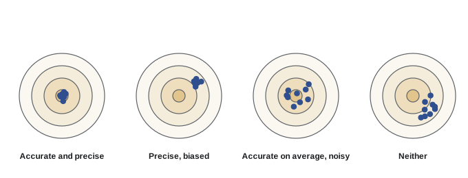
The distinction matters because the two kinds of error are fixed in different ways. Bias can often be calibrated out: measure a known reference, subtract the offset, correct the scale factor. Random noise cannot be calibrated away, but it can be reduced by averaging, filtering or fusing several sensors, at the cost of delay. Lesson 11 returns to these remedies. Resolution, finally, is usually limited by the converter and is the easiest of the three to buy more of, which is why datasheets tend to lead with it.
Worked problem
Encoder resolution at the tool
A robot joint uses a 14-bit absolute encoder on the joint output, and the tool point is 0.8 m from the joint axis. What is the smallest tool movement the encoder can detect from this joint alone?
Show solution
- A 14-bit encoder has \( 2^{14} = 16\,384 \) counts per revolution.
- Angular resolution: \( 2\pi / 16\,384 = 3.83 \times 10^{-4} \) rad.
- Arc length at 0.8 m: \( s = r\theta = 0.8 \times 3.83 \times 10^{-4} = 3.07 \times 10^{-4} \) m.
Answer: About 0.31 mm. That is the resolution, not the accuracy: gear backlash, link flex and encoder errors can make the true position error several times larger.
Dynamic characteristics
Real measurands change, and a sensor's dynamic characteristics describe how quickly and faithfully it follows them. Many sensors behave approximately like a first-order system: after a sudden step in the input, the output rises exponentially with time constant \( \tau \), reaching 63 % of the final value after one time constant and about 95 % after three. A thermistor in still air may have \( \tau \) of tens of seconds; a MEMS accelerometer responds in well under a millisecond.
The equivalent frequency-domain statement is bandwidth: the cutoff frequency \( f_c \) at which the sensor's response has fallen to about 70 % (−3 dB) of its low-frequency value. A sensor with too little bandwidth smooths away exactly the fast events, such as impacts and vibrations, that a controller may need to see. Related terms are latency (the delay between an event and the reading becoming available, which includes filtering, conversion and communication) and output data rate (how often new readings arrive). A camera might run at 30 frames per second, but if each frame takes 50 ms to expose, transfer and process, the robot always acts on a picture of the world as it was 50 ms ago.
Worked problem
Is the sensor fast enough?
A temperature sensor on a motor winding has a time constant of 4 s. The winding temperature jumps by 20 °C during a stall. How much of the rise does the sensor report after 2 s, and what is its bandwidth?
Show solution
- Fraction after 2 s: \( 1 - e^{-2/4} = 1 - 0.607 = 0.393 \).
- Reported rise: \( 0.393 \times 20 = 7.9 \) °C.
- Bandwidth: \( f_c = 1/(2\pi \times 4) = 0.040 \) Hz.
Answer: Only about 7.9 °C of the 20 °C rise after 2 s, and a bandwidth of 0.04 Hz. Thermal protection based on this sensor alone would react too slowly to a stall, which is why motor drives also estimate winding temperature from current.
Noise and the signal-to-noise ratio
Every measurement carries noise: small random fluctuations from thermal agitation in resistors, the quantum nature of light, vibration, electromagnetic interference and the converter itself. White noise has equal power at all frequencies and is described by its standard deviation \( \sigma \) for a given bandwidth, or by a noise density, such as 150 µg/√Hz for an accelerometer or 0.005 °/s/√Hz for a gyroscope. Multiplying the density by the square root of the bandwidth gives the expected standard deviation of the readings.
The second formula is the reason averaging works: the mean of N independent readings has a standard deviation \( \sqrt{N} \) times smaller. Quadrupling the number of samples halves the noise. The price is time, since averaging 16 readings from a 100 Hz sensor gives 6.25 effective readings per second, and the averaged value describes the past 0.16 s rather than the present. Averaging also does nothing for bias, which is identical in every sample.
Worked problem
Accelerometer noise at two bandwidths
An accelerometer has a noise density of 150 µg/√Hz. What noise standard deviation should you expect with a 100 Hz bandwidth, and with a 10 Hz bandwidth? (1 g = 9.81 m/s².)
Show solution
- At 100 Hz: \( \sigma = 150 \times \sqrt{100} = 1500 \) µg \( = 1.5 \) mg \( \approx 0.0147 \) m/s².
- At 10 Hz: \( \sigma = 150 \times \sqrt{10} = 474 \) µg \( \approx 0.0047 \) m/s².
- Ratio: \( \sqrt{10} \approx 3.2 \).
Answer: About 1.5 mg at 100 Hz and 0.47 mg at 10 Hz. Narrowing the bandwidth tenfold cuts the noise by about 3.2 times, but the sensor can then no longer follow fast vibration.
The signal-to-noise ratio (SNR) compares the size of the signal to the size of the noise, often in decibels: \( \text{SNR}_{\text{dB}} = 20\log_{10}(A_{\text{signal}}/A_{\text{noise}}) \) for amplitudes. A related datasheet term is dynamic range, the ratio of the largest measurable signal to the noise floor. A 16-bit converter has an ideal dynamic range of about 96 dB, but the sensor in front of it rarely achieves that.
Reading a datasheet critically
Datasheets are written by people who want to sell the part, so the numbers are true but carefully chosen. A few habits protect you. First, read the conditions: a lidar's range may be specified for a white target with 90 % reflectivity, and drop by half for a dark tire. A gyroscope's bias may be quoted at 25 °C and drift several times further over the full temperature range. Second, distinguish typical values, which half of all parts beat, from minimum or maximum values, which are guaranteed. Design with the guaranteed limits when safety depends on them. Third, check units carefully, especially for noise densities, angles (degrees versus radians) and percentages of reading versus percentages of full scale.
| Datasheet line | What it really tells you | Typical trap |
|---|---|---|
| Range 0.1–40 m | Limits for a reference target | Dark, shiny or angled surfaces may return much less |
| Accuracy ±2 cm | Error budget under stated conditions | Often excludes temperature drift and multipath |
| Resolution 1 mm | Smallest reported step | Says nothing about accuracy or noise |
| Noise density 0.005 °/s/√Hz | Random noise per root bandwidth | Multiply by √B before comparing sensors |
| Output rate 200 Hz | How often new data arrives | Latency and internal filtering may be separate |
| Operating temperature −40 to 85 °C | Where the part survives and works | Specifications may only hold near 25 °C |
Finally, an error budget combines all the contributions. Independent random errors add in quadrature (the square root of the sum of squares), while systematic errors that might all push the same way are often added directly as a worst case. If a distance sensor has 10 mm of calibration uncertainty, 6 mm of noise and 8 mm of temperature drift, the root-sum-square total is \( \sqrt{10^2 + 6^2 + 8^2} \approx 14 \) mm, whereas the worst case is 24 mm. Which number to use depends on the consequences of being wrong.
import math
# Simple error budget for a distance sensor, all values in mm
terms = {"calibration": 10.0, "noise (1 sigma)": 6.0, "temperature drift": 8.0, "mounting": 3.0}
rss = math.sqrt(sum(v**2 for v in terms.values()))
worst = sum(terms.values())
for k, v in terms.items():
    print(f"{k:18s} {v:5.1f} mm  share of variance {100*v**2/rss**2:4.1f} %")
print(f"root-sum-square total {rss:5.1f} mm")
print(f"worst-case total {worst:5.1f} mm")calibration 10.0 mm share of variance 47.8 % noise (1 sigma) 6.0 mm share of variance 17.2 % temperature drift 8.0 mm share of variance 30.6 % mounting 3.0 mm share of variance 4.3 % root-sum-square total 14.5 mm worst-case total 27.0 mm
The variance shares in the output show where effort pays off. Calibration dominates this budget, so a better calibration procedure would help more than a quieter sensor. This kind of reasoning, rather than buying the most expensive part, is what sensor selection is about, and the capstone in lesson 12 applies it to a whole robot.
Common mistakes
MistakeTreating resolution as accuracy because the sensor reports many digits.
InsteadResolution is only the step size; accuracy depends on bias, drift, nonlinearity and noise, which must be checked separately.
MistakeComparing noise densities from two datasheets without converting to the same bandwidth.
InsteadMultiply each density by the square root of the bandwidth you will actually use before comparing.
MistakeExpecting averaging to remove a constant offset.
InsteadAveraging reduces random noise by √N but leaves bias untouched; bias needs calibration against a reference.
MistakeDesigning with typical datasheet values in a safety function.
InsteadUse guaranteed minimum or maximum values across the operating temperature range when failure matters.
MistakeIgnoring latency because the output data rate is high.
InsteadA sensor can deliver 200 readings a second and still report each one 50 ms late; check delay as well as rate.
Summary and key terms
- A sensor transduces a physical measurand into a signal; the front-end physics sets its ultimate limits.
- Proprioceptive sensors measure the robot itself, exteroceptive sensors the world; active sensors emit energy, passive ones do not.
- Static characteristics include range, sensitivity, offset, resolution, linearity, hysteresis and repeatability.
- Accuracy, precision and resolution are distinct: bias limits accuracy, noise limits precision.
- Dynamic behavior is described by time constant, bandwidth, latency and output data rate.
- Noise scales with the square root of bandwidth, and averaging N samples cuts random noise by √N.
- Datasheets must be read for conditions, typical versus guaranteed values and units, then combined in an error budget.
- Transducer
- A device that converts one physical quantity into another, usually electrical.
- Proprioceptive sensor
- A sensor that measures the robot's own internal state.
- Exteroceptive sensor
- A sensor that measures the environment.
- Sensitivity
- The slope of output against input; also called scale factor.
- Bias
- A constant offset between the reading and the true value.
- Resolution
- The smallest input change that produces a detectable output change.
- Hysteresis
- Different outputs for the same input depending on the direction of change.
- Bandwidth
- The frequency range over which the sensor responds faithfully, up to the −3 dB point.
- Noise density
- Random noise per square root of bandwidth.
- Error budget
- A tally of all error sources and how they combine into a total uncertainty.
Practice problems
Work each problem on paper first, then reveal the answer to check.
Classify a wheel encoder, a camera, a battery voltage monitor and a lidar as proprioceptive or exteroceptive.
Show answer
Wheel encoder and battery monitor: proprioceptive. Camera and lidar: exteroceptive.
A 12-bit encoder sits on a motor shaft before a 50:1 gearbox. What is the output-shaft resolution?
Show answer
\( 360°/(4096 \times 50) \approx 0.0018° \), ignoring backlash.
A sensor has \( \tau = 0.2 \) s. What is its bandwidth?
Show answer
\( 1/(2\pi \times 0.2) \approx 0.80 \) Hz.
How long after a step does a first-order sensor reach about 95 % of the final value?
Show answer
About three time constants.
A gyroscope has noise density 0.01 °/s/√Hz. What is \( \sigma \) at 50 Hz bandwidth?
Show answer
\( 0.01\sqrt{50} \approx 0.071 \) °/s.
By how much does averaging 25 independent readings reduce random noise?
Show answer
By a factor of 5.
Combine errors of 3, 4 and 12 mm in quadrature.
Show answer
\( \sqrt{9 + 16 + 144} = 13 \) mm.
A scale always reads 0.5 kg high but its readings vary by only 1 g. Is it accurate, precise or both?
Show answer
Precise but not accurate.
Express an amplitude ratio of 1000 in decibels.
Show answer
\( 20\log_{10}1000 = 60 \) dB.
Why might a lidar's quoted maximum range not apply to a black car?
Show answer
Range is specified for a highly reflective reference target; dark surfaces return far less light.
Lesson quiz · 5 questions
Score 60% or more to complete this lesson.
Create a free account to save your progress, take quizzes and earn a certificate.