Tracking and 6-D pose estimation

Detection answers 'what is where in this frame'. Robots usually need more: the full position and orientation of an object in 3-D, its six-dimensional (6-D) pose, so a gripper can approach it at the right angle; and a consistent identity over time, so the robot knows the box it saw a moment ago is the same box now, and where it is heading. This lesson covers the tools for both: fiducial markers, which make pose estimation easy and reliable; the perspective-n-point problem, which computes pose from known 3-D points and their images; model- and learning-based pose estimation for ordinary objects; and multi-object tracking, which links detections across frames using the filters of ROB-310.

Fiducial markers

The most reliable way to get a camera pose in a structured environment is to put a known pattern there. Fiducial markers such as ArUco and AprilTag are black-and-white squares with a thick border and an internal binary code. Detection finds square outlines (quadrilaterals) in the image, reads the bit pattern inside, and checks it against a dictionary designed so that codes differ in many bits, giving error detection and a unique ID for each marker. Because the marker's four corners have precisely known positions on a square of side s, they give the 2-D to 3-D correspondences needed to compute the camera's pose relative to the marker in a few milliseconds.

Robots use markers to dock at chargers, to mark pick locations and shelves, to calibrate cameras and hand-eye transforms (lesson 3), to provide ground truth for testing other perception, and to localize in warehouses where a grid of ceiling or floor markers gives absolute position. The AprilTag family (from the University of Michigan) and ArUco (built into OpenCV) are both widely used, and boards of many markers give more accurate and robust poses than a single tag.

The perspective-n-point problem

Given n known 3-D points \( \mathbf{X}_j \) in an object's frame and their measured image points \( \mathbf{u}_j \), with known intrinsics K, the perspective-n-point (PnP) problem finds the rotation R and translation t that place the object relative to the camera so that the points project where they were observed. It is calibration's mirror image: there the camera parameters were unknown, here only the pose is. Three points give up to four solutions (the P3P problem), so at least four are used in practice to pick the right one; for coplanar points, such as a marker's corners, specialized solvers like IPPE exploit the plane. Efficient general solvers such as EPnP handle any number of points in linear time. As always, robust estimation with RANSAC (lesson 5) rejects bad correspondences, and a final Levenberg–Marquardt refinement minimizes reprojection error:

PnP is used everywhere: for marker poses, for camera localization against a 3-D map in visual odometry and SLAM (lesson 7), and for object poses once a network has predicted where an object's known keypoints appear in the image.

import numpy as np
rng = np.random.default_rng(21)

K = np.array([[900.0, 0, 640], [0, 900.0, 360], [0, 0, 1]])
s = 0.12                                              # marker side, m
obj = np.array([[-s/2, s/2], [s/2, s/2], [s/2, -s/2], [-s/2, -s/2]])   # corners in marker plane (z = 0)

def rot(rx, ry, rz):
    cx, sx, cy, sy, cz, sz = np.cos(rx), np.sin(rx), np.cos(ry), np.sin(ry), np.cos(rz), np.sin(rz)
    Rx = np.array([[1, 0, 0], [0, cx, -sx], [0, sx, cx]])
    Ry = np.array([[cy, 0, sy], [0, 1, 0], [-sy, 0, cy]])
    Rz = np.array([[cz, -sz, 0], [sz, cz, 0], [0, 0, 1]])
    return Rz @ Ry @ Rx

R_true = rot(np.deg2rad(25), np.deg2rad(-15), np.deg2rad(10)); t_true = np.array([0.10, -0.05, 1.50])
P3 = np.column_stack([obj, np.zeros(4)])
img = (K @ (R_true @ P3.T + t_true[:, None])).T
img = img[:, :2] / img[:, 2:] + rng.normal(0, 0.3, (4, 2))          # 0.3 px corner noise

# planar pose: homography from marker plane to image, then H = K [r1 r2 t] up to scale
A = []
for (X, Y), (u, v) in zip(obj, img):
    A += [[X, Y, 1, 0, 0, 0, -u*X, -u*Y, -u], [0, 0, 0, X, Y, 1, -v*X, -v*Y, -v]]
H = np.linalg.svd(np.array(A))[2][-1].reshape(3, 3)
B = np.linalg.inv(K) @ H
lam = 2 / (np.linalg.norm(B[:, 0]) + np.linalg.norm(B[:, 1]))
if B[2, 2] * lam < 0: lam = -lam                      # marker must be in front of the camera
r1, r2, t = lam * B[:, 0], lam * B[:, 1], lam * B[:, 2]
Rm = np.column_stack([r1, r2, np.cross(r1, r2)])
U, _, Vt = np.linalg.svd(Rm); R_est = U @ Vt          # nearest true rotation

def rodrigues(w):
    th = np.linalg.norm(w)
    if th < 1e-12: return np.eye(3)
    k = w / th; Kx = np.array([[0, -k[2], k[1]], [k[2], 0, -k[0]], [-k[1], k[0], 0]])
    return np.eye(3) + np.sin(th) * Kx + (1 - np.cos(th)) * Kx @ Kx

def residual(x):
    R = rodrigues(x[:3]) @ R_est
    q = (K @ (R @ P3.T + x[3:, None])).T
    return (q[:, :2] / q[:, 2:] - img).ravel()

def report(label, R, t):
    ang = np.degrees(np.arccos(np.clip((np.trace(R.T @ R_true) - 1) / 2, -1, 1)))
    q = (K @ (R @ P3.T + t[:, None])).T
    rms = np.sqrt(((q[:, :2] / q[:, 2:] - img) ** 2).sum(1).mean())
    e = 1000 * (t - t_true)
    print("%s: error x %.1f, y %.1f, z %.1f mm; rotation %.2f deg; RMS %.2f px" % (label, e[0], e[1], e[2], ang, rms))

report("homography only", R_est, t)

# Gauss-Newton refinement of reprojection error over a small rotation vector and t
x = np.concatenate([np.zeros(3), t])
for it in range(10):
    r0 = residual(x)
    J = np.column_stack([(residual(x + d) - r0) / 1e-6 for d in np.eye(6) * 1e-6])
    x = x - np.linalg.lstsq(J, r0, rcond=None)[0]
report("after refinement", rodrigues(x[:3]) @ R_est, x[3:])

homography only: error x -3.5, y 2.0, z -46.2 mm; rotation 7.42 deg; RMS 2.19 px
after refinement: error x -0.5, y 0.2, z -3.4 mm; rotation 1.46 deg; RMS 0.25 px

The linear homography solution is only a starting point: it leaves a 46 mm depth error, a 7° rotation error and 2.2 px of reprojection error. Refining by minimizing reprojection error, as every practical PnP solver does, brings the pose to within about 3 mm in depth and 1.5° in rotation, with residuals matching the 0.3 px corner noise. Even after refinement, the error along the viewing direction is several times the sideways error, and tilt is the least certain part of the rotation. Depth and tilt are the weak directions of single-marker pose, which is why marker boards, larger markers and filtering over several frames are used when accuracy matters.

Pose estimation for ordinary objects

Most objects do not carry markers. Several approaches estimate their 6-D pose, typically for known objects with a CAD model or a set of reference images.

• Keypoint methods train a network to predict where specific points on the object, such as corners of its 3-D bounding box or distinctive surface points, appear in the image, then solve PnP. PVNet and similar methods vote for each keypoint from many pixels, which tolerates occlusion.
• Dense correspondence methods predict, for every object pixel, its 3-D coordinate on the model, then solve PnP with RANSAC over thousands of correspondences.
• Depth-based methods match the observed point cloud against the model, using 3-D descriptors and RANSAC for a coarse pose and ICP for refinement (lesson 8). They excel with good depth and struggle on shiny or dark objects that depth sensors cannot see well.
• Render-and-compare methods refine a pose by rendering the model at the current estimate and adjusting until the rendering matches the image. Recent model-based foundation methods, such as FoundationPose, at the time of writing, generalize to new objects from a CAD model or a few images without retraining.

Pose accuracy is usually measured with the ADD metric, the average distance between model points transformed by the true and estimated poses, with a pose counted correct if ADD is below 10 % of the object's diameter; symmetric objects such as bottles and bowls use ADD-S, which takes the closest model point, because their pose is ambiguous about the symmetry axis. Symmetry deserves care in practice too: a robot gripping a cylinder does not need its angle about the axis, and forcing a network to predict it only confuses training.

Multi-object tracking

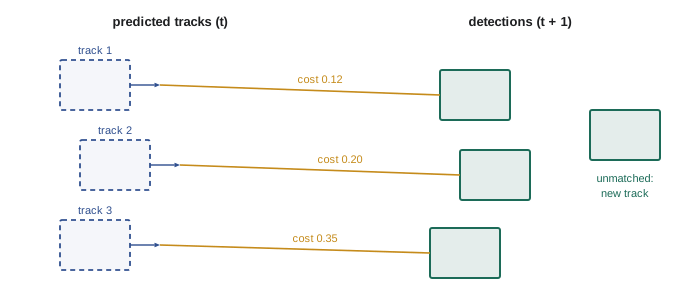
A robot watching a conveyor, a crowd or a field of plants must link detections over time into tracks, each with a persistent identity. The standard approach, tracking by detection, runs a detector on every frame and then solves a data association problem.

1. Predict each existing track forward with a motion model, usually a constant-velocity Kalman filter on the box center and size (ROB-310), giving a predicted box and its uncertainty.

2. Compute a cost between every predicted track and every new detection: 1 − IoU, a Mahalanobis distance using the predicted covariance, an appearance distance between learned embeddings, or a combination.

3. Solve the assignment with the Hungarian algorithm, which finds the matching with the lowest total cost, rejecting pairs above a gate.

4. Update matched tracks with their detections, start tentative tracks for unmatched detections, and delete tracks unmatched for too long.

SORT (2016) does this with IoU costs and a Kalman filter; DeepSORT adds an appearance embedding so identities survive occlusions; ByteTrack also associates low-confidence detections in a second pass, recovering objects that a strict threshold would drop. Tracking quality is measured with metrics such as MOTA, IDF1 and HOTA, which count misses, false positives and identity switches.

Tracking and pose together

In manipulation, tracking and pose estimation combine: a robot picking moving parts from a conveyor estimates each part's pose once with care, then tracks it with a cheap motion model (the conveyor's known speed from an encoder) and refines the pose with fast local updates, rather than solving from scratch every frame. Fusing the camera's pose estimates with a motion model in a Kalman filter also smooths jitter and lets the robot predict where the part will be when the gripper arrives, compensating for perception and planning latency (ROB-320).