Case studies and course project

This course has built a toolkit for reasoning with variable data: describing data, collecting it well, probability and distributions, reliability and extreme values, joint variation and error propagation, confidence intervals and tests, analysis of variance and designed experiments, regression and statistical quality control. Real engineering questions draw on several of these at once, and the hardest part is often deciding what question the statistics should answer. This lesson works through three case studies: setting the target strength of a concrete mix so that it passes the code acceptance rules, deciding how many tests are needed to demonstrate a reliability requirement, and judging whether an environmental change reduced air pollution. It then summarizes the habits of good statistical practice, sets out the course project and looks ahead.

Case study 1: designing concrete to pass acceptance

A structural engineer specifies a compressive strength \(f'_c\). Concrete strength varies from batch to batch, so the supplier cannot simply aim for \(f'_c\): half the tests would fall below it. ACI 318 sets the acceptance rules: for specified strengths up to 5000 psi, the average of any three consecutive strength tests must equal or exceed \(f'_c\), and no single test may fall more than 500 psi below it. This case study uses the SI edition of the rules, where the allowance is 3.5 MPa, with \(f'_c\) = 30 MPa (about 4350 psi). The supplier must choose a mean (target) strength high enough that these rules are rarely violated.

The two rules lead to two requirements. A running average of three tests has standard deviation \(s/\sqrt{3}\) (Lesson 6), so keeping its failure rate near 1% (z = 2.33) needs a mean of at least \(f'_c + 2.33s/\sqrt{3} = f'_c + 1.34s\). A single test below \(f'_c - 3.5\) MPa should also have probability about 1%, needing a mean of at least \(f'_c + 2.33s - 3.5\). The required average strength is the larger of the two, a calculation built directly into the standards.

import numpy as np

rng = np.random.default_rng(2026)
fc, s = 30.0, 3.5                         # specified strength and standard deviation (MPa)

def violations(mean, n_tests=100, years=2000):
    bad_avg = bad_single = 0
    for _ in range(years):
        x = rng.normal(mean, s, n_tests)
        avg3 = np.convolve(x, np.ones(3) / 3, mode="valid")
        bad_avg += np.sum(avg3 < fc)
        bad_single += np.sum(x < fc - 3.5)
    return bad_avg / (years * (n_tests - 2)), bad_single / (years * n_tests)

for mean in [fc, fc + 2.0, fc + 1.34 * s, fc + 6.0]:
    pa, ps = violations(mean)
    print(f"Mean {mean:5.1f} MPa: running averages below fc {100 * pa:5.2f}%, single tests below fc - 3.5: {100 * ps:5.2f}%")

Mean  30.0 MPa: running averages below fc 49.96%, single tests below fc - 3.5: 15.79%
Mean  32.0 MPa: running averages below fc 16.17%, single tests below fc - 3.5:  5.79%
Mean  34.7 MPa: running averages below fc  1.03%, single tests below fc - 3.5:  0.97%
Mean  36.0 MPa: running averages below fc  0.16%, single tests below fc - 3.5:  0.32%

At the target of 34.7 MPa, about 1% of running averages and 1% of single tests fall short, exactly as designed. Aiming at the specified strength itself fails half of the running averages. The case uses the normal distribution, the distribution of a mean, an acceptance-sampling view of risk (Lesson 11) and the control charts the supplier uses to keep s small.

Case study 2: how many tests prove reliability?

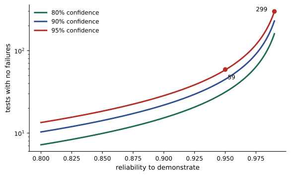
A client requires that a new valve actuator have at least 95% reliability over its duty cycle, demonstrated at 90% confidence. How many actuators must be tested? If n units are tested and none fails, the reliability R is demonstrated at confidence C when a product that only just meets the requirement would very probably have produced at least one failure, that is when \(R^n \le 1 - C\). This gives the success-run formula:

import math
from scipy import stats

# Zero-failure (success-run) demonstration: n tests, no failures, shows reliability R at confidence C
for R in [0.90, 0.95, 0.99]:
    for C in [0.90, 0.95]:
        n = math.ceil(math.log(1 - C) / math.log(R))
        print(f"Reliability {R:.2f} at {C:.0%} confidence: {n:4d} tests without failure")

# If one failure is allowed, the binomial distribution gives the required sample size
R, C = 0.95, 0.90
n = 1
while stats.binom.cdf(1, n, 1 - R) > 1 - C:
    n += 1
print(f"Allowing one failure, R = {R} at {C:.0%} confidence needs {n} tests")

Reliability 0.90 at 90% confidence:   22 tests without failure
Reliability 0.90 at 95% confidence:   29 tests without failure
Reliability 0.95 at 90% confidence:   45 tests without failure
Reliability 0.95 at 95% confidence:   59 tests without failure
Reliability 0.99 at 90% confidence:  230 tests without failure
Reliability 0.99 at 95% confidence:  299 tests without failure
Allowing one failure, R = 0.95 at 90% confidence needs 77 tests

Demonstrating 95% reliability at 90% confidence needs 45 tests with no failures; 99% at 95% needs 299. High reliability is expensive to demonstrate by testing alone, which is why engineers combine testing with physics-based analysis, accelerated life tests at higher stress (fitted with the Weibull models of Lesson 5), field data and prior experience. Allowing one failure raises the requirement to 77 tests but protects against rejecting a good design because of a single unlucky failure, a trade-off that should be agreed with the client before testing begins.

Case study 3: did a change reduce air pollution?

A city introduced measures to reduce fine particulate pollution near an industrial area. Daily average concentrations for a year before and a year after are available, and the question is whether air quality improved. Daily concentrations are positive and right-skewed, typically close to lognormal (Lesson 5), so the analysis works with logarithms. Two different summaries matter: the typical level, which affects long-term health, and the number of days above a daily limit, which the public notices.

import numpy as np
from scipy import stats

rng = np.random.default_rng(8)
limit = 25.0                                          # daily limit (micrograms per m3)
before = rng.lognormal(np.log(9.0), 0.6, 365)         # a year of daily averages before a change
after = rng.lognormal(np.log(7.8), 0.6, 365)          # a year after

for name, x in [("Before", before), ("After", after)]:
    mu, sd = np.log(x).mean(), np.log(x).std(ddof=1)
    model = stats.norm.sf((np.log(limit) - mu) / sd)
    print(f"{name}: median {np.exp(mu):.1f}, days over limit {np.sum(x > limit):2d} "
          f"(model predicts {365 * model:.1f}), 98th percentile {np.percentile(x, 98):.1f}")

# Did the change reduce typical levels? Compare the log concentrations with a two-sample t test
t, p = stats.ttest_ind(np.log(before), np.log(after))
print(f"Two-sample t test on log concentrations: t = {t:.2f}, p = {p:.2g}")
# Did it reduce exceedance days? Compare two proportions
x1, x2, n = np.sum(before > limit), np.sum(after > limit), 365
pool = (x1 + x2) / (2 * n)
z = (x1 - x2) / n / np.sqrt(pool * (1 - pool) * 2 / n)
print(f"Exceedance days {x1} vs {x2}: z = {z:.2f}, p = {2 * stats.norm.sf(abs(z)):.3f}")

Before: median 8.8, days over limit 17 (model predicts 17.2), 98th percentile 30.4
After: median 8.0, days over limit 13 (model predicts 10.5), 98th percentile 29.0
Two-sample t test on log concentrations: t = 2.25, p = 0.025
Exceedance days 17 vs 13: z = 0.75, p = 0.456

The typical (median) concentration fell by about 10%, and the t test on the logarithms shows the reduction is statistically significant. The count of days over the limit also fell, from 17 to 13, but that difference is well within chance variation: exceedances are rare events, and counting them throws away most of the information in the data. The lognormal model, fitted to all 365 days, estimates the exceedance rate more precisely, and predicts a larger relative reduction in exceedances than in the median, because a modest shift of the whole distribution removes a large share of its upper tail.

Two cautions apply. This is an observational before-and-after comparison, so weather, traffic or a change in industrial output could be responsible (Lesson 2); a better analysis includes those variables in a regression (Lesson 10) or compares with a control site that had no intervention. And one year is a short record for air quality, which varies strongly between years.

Habits of good statistical practice

Across the case studies, the same habits recur:

• Start from the engineering question, and decide in advance what result would change a decision.
• Think about how the data were collected before analyzing them; bias is not fixed by analysis.
• Plot the data first: histograms, time plots, scatter plots and probability plots reveal problems no summary will.
• Choose models for physical reasons and check their assumptions with residuals and probability plots.
• Report estimates with intervals, not just p-values, and judge practical as well as statistical significance.
• Be honest about uncertainty, multiple comparisons and the limits of observational data.
• Make the analysis reproducible: keep raw data, record each step and use scripts rather than manual edits.

The course project

Choose one of the following problems, or propose your own of similar scope with your instructor's approval. Collect or obtain real data where possible, and prepare a report with the question, data collection, analysis, checks of assumptions, results with uncertainty, and engineering conclusions.

• Project A: Designed experiment. Plan and run a small factorial experiment (for example, factors affecting the strength of a glued joint, the flight distance of a paper glider or the cooling time of a cup of water). Randomize, replicate, analyze with ANOVA, present interaction plots and recommend settings.
• Project B: Reliability. Obtain failure or life data (maintenance records, test results or a published data set). Fit exponential and Weibull models with probability plots and maximum likelihood, interpret the shape parameter, and recommend a maintenance or replacement interval.
• Project C: Process monitoring. Collect repeated measurements of a process (packaging weights, machined dimensions, daily energy use or commute times). Set up appropriate control charts, investigate any signals, and assess capability against a stated requirement.
• Project D: Regression study. Build a regression model relating an engineering response to two or more predictors (for example building energy use against temperature and occupancy, or concrete strength against water-cement ratio and age). Check residuals, give prediction intervals and discuss confounding and extrapolation.

Every report should explain how the data were collected and what biases might exist, show the key plots, state and check assumptions, give intervals for the main estimates, and end with conclusions a manager could act on.

Looking ahead

Statistics runs through engineering practice: quality engineering and Six Sigma programs, reliability and maintenance engineering, structural safety and load and resistance factor design, hydrology and environmental monitoring, transportation studies, and the growing use of data science and machine learning, which build on the regression, probability and validation ideas of this course. Later courses in numerical methods (MATH-300) supply the Monte Carlo and optimization tools for problems too complex for formulas, and design courses use the reliability concepts here to set safety factors. The central lesson carries over to all of them: every measurement and every prediction comes with uncertainty, and an engineer's job is to quantify it and design for it.