Distributions for reliability and extremes

Lesson 4 introduced the binomial, Poisson, exponential and normal distributions. They cover a great deal, but several important engineering questions need other models. How long will a bearing, a seal or a battery last, and does its failure rate rise as it ages? How long does a repair take, when most repairs are quick but a few take days? How large a flood, wind gust or snow load should a structure be designed for, when the design value is far beyond anything in the record? This lesson introduces the distributions engineers use for these questions: the Weibull distribution for component life, the lognormal distribution for quantities built up by multiplication, the gamma distribution, and the Gumbel extreme value distribution for annual maxima. Along the way it develops the language of reliability (the reliability function, the hazard rate and the bathtub curve) and shows how probability plots and maximum likelihood fit these distributions to data.

Reliability and the hazard function

For a component whose life T has density f(t) and cumulative distribution F(t), the reliability function is the probability of surviving beyond time t:

The hazard function, or instantaneous failure rate, is the rate of failure at time t among the items still working:

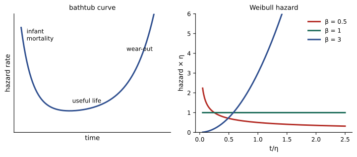
The hazard describes how aging affects failure. For the exponential distribution (Lesson 4) it is constant, \(h = \lambda\): an old component is exactly as likely to fail in the next hour as a new one, the "memoryless" property that suits random shocks and many electronic parts. Most mechanical components wear out, so their hazard rises with age; newly manufactured items often show early failures from defects, so their hazard falls at first. Combined over a product's life, these give the bathtub curve: a falling infant-mortality period, a flat useful-life period and a rising wear-out period. Burn-in testing removes the early failures before shipping; preventive replacement removes items before wear-out; and in the flat period, replacing working parts does no good at all.

The Weibull distribution

The Weibull distribution is the workhorse of reliability engineering because one parameter controls whether the hazard falls, stays constant or rises. With shape parameter β and scale parameter η (the characteristic life):

• β < 1: decreasing hazard (infant mortality, manufacturing defects).
• β = 1: constant hazard; the Weibull reduces to the exponential distribution.
• β > 1: increasing hazard (wear-out). Fatigue and bearing failures typically have β between about 1.5 and 4; at β ≈ 3.5 the distribution looks much like a normal one.

At t = η, the reliability is \(e^{-1} = 0.368\) for any β, so η is the life by which 63.2% of items have failed. Two other summaries are widely used: the mean time to failure \(\text{MTTF} = \eta\,\Gamma(1 + 1/\beta)\), using the gamma function, and the B10 life, the age by which 10% have failed, \(t_{10} = \eta(-\ln 0.9)^{1/\beta}\). Bearing manufacturers rate their products by B10 life.

A useful property follows from the formula for R. For a system of n identical components in series (Lesson 3), all of which must work, the system reliability is \(R(t)^n = e^{-n(t/\eta)^\beta}\), again a Weibull distribution with the same β but with η reduced by a factor \(n^{1/\beta}\). This weakest-link behavior is why long chains, long cables and large brittle parts are weaker on average than short ones.

Fitting a Weibull distribution

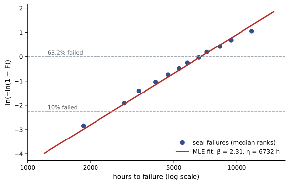
Taking logarithms twice turns the Weibull distribution function into a straight line:

So if failure times are sorted, each is given an estimated cumulative probability (the median rank \((i - 0.3)/(n + 0.4)\) for the ith of n), and the points are plotted on these axes, they should fall near a straight line whose slope is β. This Weibull probability plot is both a fitting method and a check of the model: a curved plot suggests a different distribution, a mixture of failure modes or a minimum life. The more efficient fitting method is maximum likelihood: choose the parameters that make the observed data most probable. Software does this directly, and it handles censored data, items still working when the test ended, which are common in life testing and must not simply be discarded.

import math
import numpy as np
from scipy import stats

# Hours to failure of 12 pump seals from a life test
t = np.array([1850, 2900, 3400, 4100, 4700, 5300, 5800, 6600, 7200, 8300, 9400, 11800])

# Maximum likelihood fit of a two-parameter Weibull (location fixed at zero)
beta, loc, eta = stats.weibull_min.fit(t, floc=0)
print(f"MLE:   shape beta = {beta:.2f}, scale eta = {eta:.0f} h")

# Median-rank regression on a Weibull probability plot
n = len(t)
F = (np.arange(1, n + 1) - 0.3) / (n + 0.4)            # median ranks
x, y = np.log(t), np.log(-np.log(1 - F))
slope, intercept = np.polyfit(x, y, 1)
print(f"Plot:  shape beta = {slope:.2f}, scale eta = {np.exp(-intercept / slope):.0f} h")

B10 = eta * (-np.log(0.9))**(1 / beta)
mttf = eta * math.gamma(1 + 1 / beta)
print(f"B10 life (10% failed): {B10:.0f} h;  mean time to failure: {mttf:.0f} h")
print(f"Probability a seal survives 3000 h: {np.exp(-(3000 / eta)**beta):.3f}")

MLE:   shape beta = 2.31, scale eta = 6732 h
Plot:  shape beta = 2.14, scale eta = 6768 h
B10 life (10% failed): 2541 h;  mean time to failure: 5964 h
Probability a seal survives 3000 h: 0.857

The two methods agree closely: β ≈ 2.2 to 2.3, indicating wear-out, and η ≈ 6750 h. A seal replacement interval of about 2500 h would keep in-service failures near 10%.

The lognormal distribution

If ln X is normally distributed, X has a lognormal distribution. It arises when a quantity is the product of many independent factors, just as the normal distribution arises from sums (the central limit theorem, Lesson 4). Lognormal models fit repair times, particle sizes, fatigue lives at a given stress, soil permeability, pollutant concentrations and the sizes of many natural quantities. They are always positive and skewed to the right: most values are moderate, a few are very large.

Calculations are done on the logarithms. If ln X has mean μ and standard deviation σ, the median of X is \(e^{\mu}\), and its mean is \(e^{\mu + \sigma^2/2}\), larger than the median because of the long right tail.

The gamma distribution

The time until the kth event of a Poisson process with rate λ (Lesson 4) follows a gamma distribution with shape k and rate λ: it is the sum of k independent exponential waiting times, with mean k/λ. More generally the gamma distribution, with any positive shape, is a flexible model for positive, right-skewed quantities such as rainfall totals, the time to complete a multi-stage task, or the load accumulated by several independent events. For example, if a standby system can absorb three component failures and failures occur at a rate of one per 1000 h, the time to exhausting the spares is gamma with k = 3 and mean 3000 h.

Extreme values: designing for the rare event

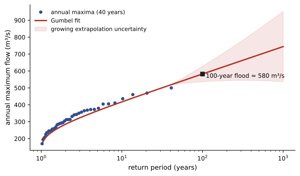
Structures must withstand the largest flood, wind gust, snow load or earthquake they are likely to see in their lifetime, and these maxima follow their own distributions. The maximum of many independent values tends toward one of a few extreme value distributions, of which the Gumbel distribution is the most widely used for annual maximum floods, winds and loads:

where the parameters u and a are estimated here from the mean \(\bar{x}\) and standard deviation s of the annual maxima (the method of moments). The T-year return level, the value exceeded on average once in T years (Lesson 3), is the value with \(F(x_T) = 1 - 1/T\):

Choosing a distribution

Physical reasoning should guide the choice: Weibull for weakest-link failure and wear-out, exponential for random failures with no aging, lognormal for multiplicative processes, gamma for sums of waiting times, Gumbel and related distributions for maxima, and normal for sums and measurement errors. Then check the choice against data with probability plots, and remember that distributions that fit equally well in the middle of the data can differ greatly in the tails, which is exactly where design decisions are made. When the tail matters, test the sensitivity of the decision to the choice of distribution.