Collecting data: sampling, measurement and experimental design

Lesson 1 showed how to summarize data once you have it. The quality of any statistical conclusion, however, is decided earlier: by how the data were collected. A sample chosen for convenience can be biased in ways no calculation can repair; a gauge that cannot tell good parts from bad makes every later test meaningless; and an experiment that changes two things at once cannot say which one mattered. This lesson covers the decisions an engineer makes before the first number is recorded. It compares the main sampling methods and the biases that creep into samples, explains how to judge a measurement system by its accuracy, precision, repeatability and reproducibility, distinguishes observational studies from experiments, and sets out the principles of experimental design (control, randomization, replication and blocking) that the analysis methods of Lessons 8 and 9 rely on. It ends with practical rules for recording and cleaning data.

Why the collection method matters

Statistics can quantify random error, the scatter that comes from chance, and shrink it by taking larger samples. It cannot detect or remove systematic error, or bias, which pushes every result the same way. A sample of 1000 biased measurements gives a very precise estimate of the wrong value. The classic engineering examples are mundane: testing only the concrete trucks that arrived on time, inspecting only the parts at the top of a bin, surveying only the customers who answered the phone, or taking water samples only on dry days. Each produces a sample that differs systematically from the population it is meant to represent.

Sampling methods

The aim of sampling is a sample whose composition mirrors the population, chosen so that the uncertainty of the estimates can be calculated. Four methods cover most engineering situations:

• Simple random sampling: every possible sample of size n is equally likely. Number the items and use random numbers to pick them. It is the basis of most statistical formulas.
• Stratified sampling: divide the population into groups (strata) that differ from one another, such as suppliers, shifts or production lines, and take a random sample from each, usually in proportion to its size. It guarantees that every group is represented and, when groups differ, gives more precise estimates than a simple random sample of the same size.
• Systematic sampling: take every kth item from a sequence, such as every 50th part off a line or a core every 100 m along a road, starting at a random point. It is easy to carry out and spreads the sample evenly, but it can be badly misled if the process has a cycle that matches k.
• Cluster sampling: pick a few groups at random and measure everything in them, such as all the bolts in three randomly chosen boxes. It is cheap when travel or handling is the main cost, but items within a cluster tend to be alike, so it is less precise than its sample size suggests.

import numpy as np

rng = np.random.default_rng(42)
# A lot of 3000 bolts from three suppliers with different mean tensile strengths (MPa)
sizes, means = [1500, 1000, 500], [830, 860, 900]
lot = np.concatenate([rng.normal(m, 12, n) for m, n in zip(means, sizes)])
supplier = np.repeat([0, 1, 2], sizes)
true_mean = lot.mean()

srs, strat = [], []
for _ in range(10000):
    srs.append(rng.choice(lot, 30, replace=False).mean())
    # stratified: 15, 10 and 5 bolts, in proportion to each supplier share
    parts = [rng.choice(lot[supplier == s], k, replace=False) for s, k in zip(range(3), [15, 10, 5])]
    strat.append(np.concatenate(parts).mean())

print(f"True lot mean: {true_mean:.1f} MPa")
print(f"Simple random samples of 30: mean {np.mean(srs):.1f}, spread (SD) {np.std(srs):.2f} MPa")
print(f"Stratified samples of 30:    mean {np.mean(strat):.1f}, spread (SD) {np.std(strat):.2f} MPa")
first = lot[:30].mean()
print(f"First 30 bolts off the pile (all from one supplier): {first:.1f} MPa")

True lot mean: 851.4 MPa
Simple random samples of 30: mean 851.4, spread (SD) 5.21 MPa
Stratified samples of 30:    mean 851.3, spread (SD) 2.16 MPa
First 30 bolts off the pile (all from one supplier): 830.2 MPa

Sources of bias

Even with a good sampling plan, bias can enter in several ways, and recognizing them is half of preventing them:

• Selection bias: the way items are chosen favors some over others, as with convenience samples or volunteers.
• Non-response or missing-data bias: some selected items are never measured, and the missing ones differ from the rest. Specimens that broke during handling, survey forms not returned, and sensors that fail in extreme conditions are all examples.
• Measurement bias: the instrument or procedure reads consistently high or low, for example an uncalibrated load cell or a technician who rounds readings toward a target.
• Survivorship bias: only items that survived some process are observed. Studying the bridges still standing tells you little about why others failed.

Writing down how each sample was chosen, and who chose it, is the simplest defense: it lets a reviewer spot problems that the person collecting the data did not.

Measurement systems

Every measurement is the true value plus error. Two properties describe a measurement system. Accuracy (or trueness) is how close the average reading is to the true value; its opposite is bias, which is found and corrected by calibration against a reference standard. Precision is how close repeated readings are to each other, measured by their standard deviation. A gauge can be precise but inaccurate (tightly grouped readings in the wrong place) or accurate but imprecise (centered but scattered).

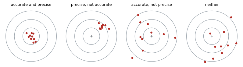
Precision is often split further. Repeatability is the variation when the same operator measures the same part repeatedly with the same gauge; reproducibility is the extra variation between operators, labs or set-ups. A gauge repeatability and reproducibility (gauge R&R) study, in which several operators measure several parts several times, estimates both, using the analysis of variance of Lesson 9. A common rule of thumb compares the measurement standard deviation with the tolerance: if the measurement system uses up more than about 30% of the tolerance, it cannot reliably separate good parts from bad.

Resolution matters too. A gauge should read to about one tenth of the tolerance or of the process spread; a caliper reading to 0.1 mm cannot police a tolerance of ±0.05 mm.

Observational studies and experiments

In an observational study, the engineer records what happens without intervening: the pavement condition on roads with different traffic, the failure rates of pumps in different plants. In an experiment, the engineer deliberately sets the conditions, such as the curing temperature of concrete or the cutting speed of a tool, and observes the response. Only experiments can establish cause and effect convincingly.

The reason is confounding. In observational data, the factor of interest is often tangled with others. Roads with heavy traffic may also be older and in wetter areas; pumps in one plant may also run harder and get less maintenance. A difference in outcomes cannot then be attributed to any one factor. Observational studies are still valuable, often the only option for large or historical systems, but their conclusions about causes must be cautious, and they should record as many potential confounding variables as possible so that the analysis can account for them (for example with the multiple regression of Lesson 10).

Principles of experimental design

A well-designed experiment answers its question with the fewest runs and with conclusions that can be trusted. Four principles do most of the work:

• Control: hold everything constant except the factors being studied, and include a baseline or control condition for comparison.
• Randomization: assign treatments to experimental units, and decide the run order, at random. This spreads the effects of unknown or uncontrollable variables (drifting room temperature, a tiring operator, a gradually wearing tool) evenly across treatments, so they cannot masquerade as treatment effects.
• Replication: run each treatment on several independent units. Replication measures the natural variation, without which no test of significance is possible, and reduces the uncertainty of each treatment mean. Measuring the same specimen three times is repeated measurement, not replication.
• Blocking: when units come in groups known to differ, such as batches of material, days or machines, compare treatments within each group. Differences between blocks then drop out of the comparison, as in the paired t-test of Lesson 7.

When several factors may matter, changing one factor at a time is inefficient and misses interactions, cases where the effect of one factor depends on the level of another. Factorial designs, which vary all factors together in a planned pattern, are the subject of Lesson 9.

Recording and cleaning data

Good data management prevents many errors. Record raw measurements, not just summaries, together with units, dates, instrument identifiers, operators and any unusual conditions. Keep the original record unchanged and do any cleaning in a copy, with each change documented. Check for impossible values (negative lengths, strengths ten times typical), duplicated entries, unit mix-ups and transcription errors. Investigate outliers (Lesson 1) rather than deleting them: an outlier may be a recording mistake, but it may also be the most important observation in the data set, such as the first sign of a process going wrong. Removing inconvenient points to obtain a desired result is scientific misconduct, and in safety-critical work it can be dangerous.