
CMPUT-204 · Lesson 1 of 12 · 29 min
What algorithms are and how we analyse them
An algorithm is a finite, precise sequence of steps that transforms an input into an output and always stops. CMPUT-174 introduced algorithms as recipes and CMPUT-201 showed how to express them in C. This course asks two harder questions about every algorithm: is it correct for every valid input, and how much time and memory does it use as the input grows? Answering those questions with mathematics rather than guesswork is what lets a computing scientist predict, before writing any code, that one approach will finish in a second and another will run for a century.
Problems, instances and algorithms
A computational problem describes a relationship between inputs and outputs. The sorting problem, for example, says: given a sequence of \(n\) comparable items, output the same items in non-decreasing order. A particular input, such as the list 5, 2, 9, 1, is an instance of the problem. An algorithm solves the problem if, for every instance, it halts with a correct output. One wrong answer on one instance is enough to make an algorithm incorrect, which is why the proof techniques from CMPUT-272 matter here: testing samples instances, but a proof covers all of them.
Most problems can be solved by many different algorithms. Sorting alone has dozens of well-known methods, and they differ enormously in speed. The study of algorithms is largely the study of these differences: which designs are possible, which are fastest for which inputs, and which limits no algorithm can beat. A problem also has a size, written \(n\), that measures how big an instance is. For sorting, \(n\) is the number of items; for a graph problem it may be the numbers of vertices and edges, written \(n\) and \(m\); for arithmetic on big numbers it is the number of digits.
| Problem | Instance | Size measure | Output |
|---|---|---|---|
| Sorting | A list of n keys | n, the number of keys | The keys in order |
| Searching a sorted list | A sorted list and a target | n, the list length | An index or not found |
| Shortest path | A weighted graph and two vertices | n vertices and m edges | A cheapest route |
| Multiplication | Two integers | n, the number of digits | Their product |
| Scheduling | A set of tasks with times | n, the number of tasks | A conflict-free plan |
A model of computation
To compare algorithms independently of any particular laptop, we use an abstract machine called the random-access machine, or RAM model. In this model, each simple operation takes one unit of time: an arithmetic operation on a machine-sized number, a comparison, an assignment, reading or writing one array cell, following a pointer, or calling and returning from a function. Memory is a large array of cells, and any cell can be reached in one step by its address. Loops and function calls are not simple operations; their cost is the sum of the operations they perform.
The RAM model ignores caches, pipelines and the difference between a fast and a slow processor. That sounds like a serious simplification, and it is, but it captures what usually matters most: how the number of steps grows with the input. A real computer might run each step ten times faster than another, yet if one algorithm needs \(n^2\) steps and the other \(n \log_2 n\), the second wins by a margin that grows without limit as \(n\) grows. Constant factors still matter in practice, and lesson 12 returns to them, but growth rate is the first thing to get right.
Correctness first
Speed is worthless if the output is wrong, so every algorithm in this course comes with an argument that it is correct. For loops, the main tool is the loop invariant from CMPUT-272 lesson 12: a statement that holds before the loop, is maintained by each iteration, and together with the exit condition implies the result. For recursive algorithms, the tool is induction on the input size: assume the recursive calls are correct on smaller inputs and show the combination is correct. For greedy algorithms, lesson 11 introduces exchange arguments. You will see all three repeatedly.
Counting operations
To analyse running time, we count the basic operations an algorithm performs as a function of \(n\), usually focusing on one dominant operation, such as key comparisons in sorting. Consider the problem of deciding whether a list contains a duplicate. The simplest algorithm compares every pair of positions. With \(n\) items there are \(n(n-1)/2\) pairs, so in the worst case, when there is no duplicate, the algorithm makes \(n(n-1)/2\) comparisons.
def has_duplicate_pairs(xs):
    """Compare every pair; return (answer, comparisons)."""
    comps = 0
    n = len(xs)
    for i in range(n):
        for j in range(i + 1, n):
            comps += 1
            if xs[i] == xs[j]:
                return True, comps
    return False, comps

def has_duplicate_sorted(xs):
    """Sort a copy, then compare adjacent items; counts only the scan."""
    ys = sorted(xs)
    comps = 0
    for i in range(len(ys) - 1):
        comps += 1
        if ys[i] == ys[i + 1]:
            return True, comps
    return False, comps

for n in (10, 100, 1000):
    data = list(range(n))            # worst case: no duplicate
    a, c1 = has_duplicate_pairs(data)
    b, c2 = has_duplicate_sorted(data)
print(n, a, c1, n * (n - 1) // 2, b, c2)10 False 45 45 False 9 100 False 4950 4950 False 99 1000 False 499500 499500 False 999
The pairwise algorithm's count matches the formula exactly: 45, 4,950 and 499,500. The second algorithm sorts first, which costs about \(n \log_2 n\) comparisons with a good sorting method (lessons 4 and 5), and then scans adjacent pairs, which costs \(n-1\) more. For \(n = 1000\), that is roughly 10,000 plus 999 comparisons instead of half a million. A third approach, inserting items into a hash set as in CMPUT-201 lesson 9, uses expected constant time per item and so about \(n\) operations in total, at the cost of extra memory.
Best, worst and average case
The number of steps often depends on the particular instance, not just its size. The pairwise duplicate check stops after one comparison if the first two items are equal, but needs all \(n(n-1)/2\) comparisons if there is no duplicate. We therefore distinguish three measures. The worst-case running time \(T(n)\) is the maximum number of steps over all instances of size \(n\). The best case is the minimum. The average case is the expected number of steps when instances are drawn from some probability distribution, which must be stated.
Worst-case analysis is the default in this course, for three reasons. It is a guarantee: no input of size \(n\) will take longer. Worst cases happen in practice more often than people expect, for instance when an adversary chooses the input or when real data is already sorted. And average-case analysis depends on an assumption about the input distribution that may not hold. Best-case analysis is rarely useful on its own, because almost any algorithm can be made fast on some lucky input.
Worked problem
Worst and best case of linear search
Linear search scans a list of n items from the left and stops at the first match. Count comparisons in the best case, the worst case and the average case when the target is present and equally likely to be at each position.
Show solution
- Best case: the target is at position 0, so 1 comparison.
- Worst case: the target is absent or last, so n comparisons.
- Average case: if the target is at position i (counting from 1) the search uses i comparisons; each position has probability 1/n.
- Expected comparisons = (1 + 2 + ... + n)/n = (n(n + 1)/2)/n = (n + 1)/2.
Answer: Best 1, worst n, average (n + 1)/2. The average is about half the worst case, so both grow linearly with n.
Why growth rate dominates
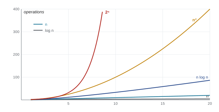
The table below shows how several common running-time functions grow. Assume a computer that performs a billion basic operations per second. An algorithm that needs \(n \log_2 n\) operations sorts a million items in about 0.02 seconds. An algorithm that needs \(n^2\) operations takes about 17 minutes for the same input, and one that needs \(2^n\) operations cannot even finish \(n = 100\) before the Sun burns out.
import math
funcs = [('log2 n', lambda n: math.log2(n)), ('n', lambda n: n),
         ('n log2 n', lambda n: n * math.log2(n)), ('n^2', lambda n: n ** 2),
         ('n^3', lambda n: n ** 3)]
ops_per_second = 1e9
for n in (10**3, 10**6, 10**9):
    row = []
    for name, f in funcs:
        secs = f(n) / ops_per_second
        row.append(f'{name}: {secs:.3g} s')
print(f'n = {n:>10}:', ', '.join(row))n = 1000: log2 n: 9.97e-09 s, n: 1e-06 s, n log2 n: 9.97e-06 s, n^2: 0.001 s, n^3: 1 s n = 1000000: log2 n: 1.99e-08 s, n: 0.001 s, n log2 n: 0.0199 s, n^2: 1e+03 s, n^3: 1e+09 s n = 1000000000: log2 n: 2.99e-08 s, n: 1 s, n log2 n: 29.9 s, n^2: 1e+09 s, n^3: 1e+18 s
Two lessons follow from the table. First, improving an algorithm's growth rate can matter far more than buying a faster computer: a machine 1,000 times faster lets an \(n^2\) algorithm handle only about 32 times more data in the same time, since \(\sqrt{1000} \approx 31.6\), while switching to an \(n \log n\) algorithm makes the same problem nearly instant. Second, for small \(n\) the differences are tiny, so a simple algorithm is often the right choice for small inputs. Real sorting libraries combine both ideas, as lesson 12 explains.
| Running time | Name | Typical source |
|---|---|---|
| 1 | Constant | Array indexing, arithmetic on one number |
| log n | Logarithmic | Halving the problem each step, as in binary search |
| n | Linear | One pass over the input |
| n log n | Linearithmic | Divide and conquer with linear merging, efficient sorting |
| n² | Quadratic | All pairs of items, nested loops |
| n³ | Cubic | All triples, naive matrix multiplication |
| 2ⁿ | Exponential | Trying every subset |
| n! | Factorial | Trying every ordering |
Measuring in practice
Counting operations predicts growth; measuring wall-clock time checks the prediction on real hardware. Timings are noisy: other programs compete for the processor, caches warm up, and Python's interpreter adds overhead to every step. Good practice is to repeat each measurement several times, report the minimum or median, use input sizes that differ by a constant factor, and look at ratios. If an algorithm is quadratic, doubling \(n\) should roughly quadruple the time; if it is linearithmic, the ratio should be a little over two.
import time, random

def time_it(f, data, repeats=5):
    best = float('inf')
    for _ in range(repeats):
        start = time.perf_counter()
        f(data)
        best = min(best, time.perf_counter() - start)
    return best

random.seed(1)
for n in (2000, 4000, 8000):
    data = [random.random() for _ in range(n)]
    print(n, time_it(sorted, data))   # ratios near 2.1 suggest n log n
The listing above is not run on this page because its output changes every time. When you run it yourself, expect each doubling of \(n\) to slightly more than double the time for Python's built-in sort. A doubling experiment is a quick way to spot an accidental quadratic algorithm hiding in code that should be linear, a common performance bug that lesson 12 discusses further.
How this course is organized
Lessons 2 and 3 build the mathematical tools: asymptotic notation and the analysis of loops and recurrences. Lessons 4 to 6 apply them to sorting and to divide and conquer, ending with a proof that no comparison sort can beat \(n \log n\). Lessons 7 to 10 turn to graphs: searching, ordering, shortest paths and minimum spanning trees. Lesson 11 develops greedy algorithms and how to prove them correct, and lesson 12 brings everything together in a design problem. Dynamic programming, network flow, NP-completeness and randomized algorithms continue in CMPUT-304; path planning for robots in ROB-310 and ROB-340 builds on the graph lessons here.
Worked problem
Choosing between two algorithms
Algorithm A takes 100n log₂ n steps and algorithm B takes n² steps. For which n is A faster?
Show solution
- A is faster when 100n log₂ n < n², that is, when 100 log₂ n < n.
- Try n = 512: 100 × 9 = 900 > 512, so B is faster.
- Try n = 1024: 100 × 10 = 1000 < 1024, so A is faster.
- Checking values in between shows the crossover lies between 996 and 997; above it A wins by a growing margin.
Answer: A is faster for every n of about 1,000 or more. Below that, B's smaller constant wins, which is why libraries switch to simple methods for small inputs.
Common mistakes
MistakeJudging an algorithm by how fast it ran on one test input.
InsteadAnalyse the worst case as a function of n, and confirm growth with a doubling experiment over several sizes.
MistakeCounting a loop as one step.
InsteadA loop costs the sum of the work in all its iterations; a call to a library function such as sorted costs whatever that function does.
MistakeAssuming the average case unless stated otherwise.
InsteadUse worst-case analysis by default; an average case is only meaningful once the input distribution is specified.
MistakeThinking a faster computer fixes a slow algorithm.
InsteadA constant-factor speed-up cannot compensate for a worse growth rate once n is large.
MistakeIgnoring correctness while optimizing speed.
InsteadEstablish correctness with an invariant or induction first; a fast wrong answer is still wrong.
Summary and key terms
- An algorithm solves a problem if it halts with a correct output on every instance; testing samples instances, proof covers all of them.
- The size n of an instance depends on the problem: items, vertices and edges, or digits.
- The RAM model charges one unit for each simple operation, which lets us compare algorithms independently of hardware.
- Worst-case running time is the default measure because it is a guarantee that does not depend on assumptions about inputs.
- Linear search uses 1 comparison in the best case, n in the worst and (n + 1)/2 on average when the target is present.
- Growth rate dominates constant factors for large n, so n log n beats n² by a margin that grows without bound.
- Doubling experiments check predicted growth on real machines; timings are noisy, so repeat them and look at ratios.
- Algorithm
- A finite, precise procedure that halts with an output for every valid input.
- Instance
- One particular input to a problem.
- Input size
- A measure n of how big an instance is, used to express running time.
- RAM model
- An abstract machine in which simple operations and memory accesses each take one unit of time.
- Worst case
- The maximum running time over all inputs of a given size.
- Average case
- The expected running time over a stated distribution of inputs of a given size.
- Best case
- The minimum running time over all inputs of a given size.
- Basic operation
- The operation counted in an analysis, such as a key comparison.
- Growth rate
- How a running-time function increases as n increases, ignoring constant factors.
- Doubling experiment
- Timing an algorithm at sizes n, 2n, 4n and comparing ratios to infer its growth rate.
Practice problems
Work each problem on paper first, then reveal the answer to check.
How many comparisons does the pairwise duplicate check make on a list of 20 distinct items?
Show answer
20 × 19 / 2 = 190.
Name the input size you would use for multiplying two large integers.
Show answer
The number of digits (or bits) in the integers.
Why is best-case analysis rarely informative?
Show answer
Almost any algorithm is fast on some lucky input, so the best case says little about what users will experience.
An algorithm doubles in time each time n increases by 1. What growth rate does that suggest?
Show answer
Exponential, about 2ⁿ.
In a doubling experiment, the time goes from 1.0 s to 4.1 s to 16.3 s. What growth rate fits?
Show answer
Quadratic: each doubling multiplies the time by about 4.
Linear search on 1,000 items where the target is present and equally likely anywhere: expected comparisons?
Show answer
(1000 + 1)/2 = 500.5.
At 10⁹ operations per second, roughly how long does an n² algorithm take for n = 10⁶?
Show answer
10¹² operations, about 1,000 seconds or 17 minutes.
Algorithm A uses 50n steps and B uses n²/2. For which n is A faster?
Show answer
When 50n < n²/2, that is, n > 100.
Which proof technique suits a recursive algorithm?
Show answer
Induction on the input size, assuming the recursive calls are correct for smaller inputs.
Give one reason worst-case analysis is preferred.
Show answer
It is a guarantee for every input of that size; or it does not depend on an assumed input distribution; or adversarial and sorted inputs make bad cases common.
Lesson quiz · 5 questions
Score 60% or more to complete this lesson.
Create a free account to save your progress, take quizzes and earn a certificate.